Of course! Here is a comprehensive guide on how to implement a Support Vector Machine (SVM) in Python using the cvxopt library.
Why cvxopt for SVM?
While popular libraries like scikit-learn provide off-the-shelf SVM implementations (sklearn.svm.SVC), learning to build an SVM from scratch using cvxopt is incredibly valuable for several reasons:
- Understanding the Math: It forces you to understand the underlying Quadratic Programming (QP) problem that SVMs solve.
- Full Control: You can implement different types of SVMs (linear, non-linear with custom kernels) without being limited by a library's API.
- Foundation for Advanced Topics: It's the perfect starting point for understanding more complex models like Support Vector Regression (SVR) or Structured SVMs.
We will implement a non-linear SVM with a Radial Basis Function (RBF) kernel, which is one of the most common and powerful types of SVMs.
The Core Idea: The SVM Optimization Problem
A binary SVM aims to find the optimal hyperplane that separates two classes of data with the maximum margin. For non-linearly separable data, we use the "kernel trick" to map the data into a higher-dimensional space where it becomes linearly separable.
The problem can be formulated as a Quadratic Program (QP):
Minimize:
½ * wᵀw + C * Σ(ξᵢ)
Subject to:
yᵢ(xᵢᵀw + b) ≥ 1 - ξᵢ for all i
ξᵢ ≥ 0 for all i
Where:
wis the weight vector.bis the bias term.- are the "slack variables," which allow for some misclassification.
Cis a hyperparameter that controls the trade-off between maximizing the margin and minimizing the classification error. yᵢare the labels (+1or-1).xᵢare the data points.
This QP problem needs to be reformulated into the standard form that cvxopt can solve:
Minimize:
½ * xᵀ * P * x + qᵀ * x
Subject to:
G * x ≤ h
A * x = b
Our goal is to map the SVM problem to these variables (P, q, G, h, A, b).
Step-by-Step Implementation with cvxopt
Step 1: Install cvxopt
If you don't have it installed, open your terminal or command prompt and run:
pip install cvxopt numpy matplotlib
Step 2: Generate a Non-Linear Dataset
We'll use scikit-learn to generate a "moons" dataset, which is not linearly separable in its original 2D space.
import numpy as np
from sklearn.datasets import make_moons
import matplotlib.pyplot as plt
# Generate a non-linear dataset
X, y = make_moons(n_samples=100, noise=0.1, random_state=42)
# Convert labels from {0, 1} to {-1, 1}
y = np.where(y == 0, -1, 1)
# Visualize the data
plt.scatter(X[:, 0], X[:, 1], c=y, cmap='viridis')"Non-Linearly Separable Data")
plt.show()
Step 3: Define the Kernel Function
The kernel function computes the dot product between data points in the (implicit) higher-dimensional space. The RBF (Gaussian) kernel is a popular choice.
def rbf_kernel(X1, X2, gamma=1.0):
    """
    Computes the RBF kernel matrix between two sets of vectors.
    K(x_i, x_j) = exp(-gamma * ||x_i - x_j||^2)
    """
    # Calculate the squared Euclidean distance matrix
    sq_dist = np.sum(X1**2, axis=1).reshape(-1, 1) + np.sum(X2**2, axis=1) - 2 * np.dot(X1, X2.T)
    # Compute the RBF kernel matrix
    K = np.exp(-gamma * sq_dist)
    return K
Step 4: Set up the Quadratic Programming Problem
This is the most critical step. We need to define the matrices P, q, G, h, A, and b for the cvxopt solver based on our dual SVM problem.
The dual problem is often easier to solve and is where the kernel trick is applied directly.
import cvxopt
def svm_fit(X, y, C=1.0, gamma=1.0):
    """
    Solves the dual SVM optimization problem using cvxopt.
    """
    n_samples, n_features = X.shape
    # Calculate the kernel matrix
    K = rbf_kernel(X, X, gamma)
    # Set up the QP problem matrices for cvxopt
    # P = y_i y_j K(x_i, x_j)
    P = cvxopt.matrix(np.outer(y, y) * K)
    q = cvxopt.matrix(np.ones(n_samples) * -1)
    # Constraints: y_i α_i = 0
    # A = y, b = 0
    A = cvxopt.matrix(y, (1, n_samples), 'd')
    b = cvxopt.matrix(0.0)
    # Constraints: 0 <= α_i <= C
    # G = [-I, I], h = [0, C]
    G_top = -np.eye(n_samples)
    G_bottom = np.eye(n_samples)
    G = cvxopt.matrix(np.vstack((G_top, G_bottom)))
    h_top = np.zeros(n_samples)
    h_bottom = np.ones(n_samples) * C
    h = cvxopt.matrix(np.hstack((h_top, h_bottom)))
    # Solve the QP problem
    solution = cvxopt.solvers.qp(P, q, G, h, A, b)
    # Extract the Lagrange multipliers (alpha)
    alphas = np.array(solution['x']).flatten()
    # Find the support vectors (where alpha > 1e-5)
    sv_indices = alphas > 1e-5
    support_vectors = X[sv_indices]
    support_vector_alphas = alphas[sv_indices]
    support_vector_labels = y[sv_indices]
    # Calculate the bias (b)
    # b = y_j - Σ(α_i y_i K(x_i, x_j)) for any support vector x_j
    # We average over all support vectors for numerical stability
    b = 0
    for i in range(len(support_vector_alphas)):
        b += support_vector_labels[i]
        b -= np.sum(support_vector_alphas * support_vector_labels * rbf_kernel(support_vectors, support_vectors[i:i+1], gamma))
    b /= len(support_vector_alphas)
    return support_vectors, support_vector_alphas, support_vector_labels, b, gamma
Step 5: Train the SVM Model
Now, we can call our svm_fit function to train the model.
# Hyperparameters
C = 10.0       # Regularization parameter
gamma = 1.0    # Kernel parameter for RBF
# Train the SVM
support_vectors, alphas, sv_labels, b, gamma = svm_fit(X, y, C, gamma)
print(f"Number of Support Vectors: {len(support_vectors)}")
print(f"Bias (b): {b}")
Step 6: Make Predictions
To predict the class of a new data point x_new, we use the "decision function":
f(x_new) = sign( Σ(α_i * y_i * K(x_i, x_new)) + b )
def svm_predict(X_new, support_vectors, alphas, sv_labels, b, gamma):
    """
    Predicts the class of new data points.
    """
    # Calculate the kernel between new points and support vectors
    K = rbf_kernel(X_new, support_vectors, gamma)
    # Calculate the decision function
    decision_function = np.dot((alphas * sv_labels), K.T) + b
    # Predict the class (sign of the decision function)
    predictions = np.sign(decision_function)
    return predictions
# Example: Predict on the original dataset
predictions = svm_predict(X, support_vectors, alphas, sv_labels, b, gamma)
# Calculate accuracy
accuracy = np.mean(predictions == y)
print(f"Training Accuracy: {accuracy * 100:.2f}%")
Step 7: Visualize the Results
Visualizing the decision boundary and the support vectors is key to understanding how the SVM works.
def plot_svm_boundary(X, y, support_vectors, b, gamma):
    """
    Plots the data points, support vectors, and decision boundary.
    """
    plt.scatter(X[:, 0], X[:, 1], c=y, cmap='viridis', s=50, edgecolors='k')
    # Highlight support vectors
    plt.scatter(support_vectors[:, 0], support_vectors[:, 1], s=200, facecolors='none', edgecolors='r', linewidths=2, label='Support Vectors')
    # Create a grid to plot the decision boundary
    x_min, x_max = X[:, 0].min() - 1, X[:, 0].max() + 1
    y_min, y_max = X[:, 1].min() - 1, X[:, 1].max() + 1
    xx, yy = np.meshgrid(np.arange(x_min, x_max, 0.02),
                         np.arange(y_min, y_max, 0.02))
    # Predict on the grid
    grid_points = np.c_[xx.ravel(), yy.ravel()]
    Z = svm_predict(grid_points, support_vectors, alphas, sv_labels, b, gamma)
    Z = Z.reshape(xx.shape)
    # Plot decision boundary and margins
    plt.contour(xx, yy, Z, levels=[-1, 0, 1], linestyles=['--', '-', '--'], colors=['k', 'k', 'k'])
    plt.title("SVM with RBF Kernel")
    plt.xlabel("Feature 1")
    plt.ylabel("Feature 2")
    plt.legend()
    plt.show()
plot_svm_boundary(X, y, support_vectors, b, gamma)
You should see a plot where the data points are colored by their true class, the support vectors are circled, and the solid line is the decision boundary, with the dashed lines indicating the margin.
Full Code
Here is the complete, runnable script for your convenience.
import numpy as np
from sklearn.datasets import make_moons
import cvxopt
import cvxopt.solvers
import matplotlib.pyplot as plt
# --- 1. Generate Data ---
X, y = make_moons(n_samples=100, noise=0.1, random_state=42)
y = np.where(y == 0, -1, 1)
# --- 2. Kernel Function ---
def rbf_kernel(X1, X2, gamma=1.0):
    sq_dist = np.sum(X1**2, axis=1).reshape(-1, 1) + np.sum(X2**2, axis=1) - 2 * np.dot(X1, X2.T)
    return np.exp(-gamma * sq_dist)
# --- 3. SVM Fitting Function ---
def svm_fit(X, y, C=1.0, gamma=1.0):
    n_samples, n_features = X.shape
    K = rbf_kernel(X, X, gamma)
    # Set up QP matrices for cvxopt
    P = cvxopt.matrix(np.outer(y, y) * K)
    q = cvxopt.matrix(np.ones(n_samples) * -1)
    A = cvxopt.matrix(y, (1, n_samples), 'd')
    b = cvxopt.matrix(0.0)
    G_top = -np.eye(n_samples)
    G_bottom = np.eye(n_samples)
    G = cvxopt.matrix(np.vstack((G_top, G_bottom)))
    h_top = np.zeros(n_samples)
    h_bottom = np.ones(n_samples) * C
    h = cvxopt.matrix(np.hstack((h_top, h_bottom)))
    # Solve QP problem
    solution = cvxopt.solvers.qp(P, q, G, h, A, b)
    alphas = np.array(solution['x']).flatten()
    # Find support vectors
    sv_indices = alphas > 1e-5
    support_vectors = X[sv_indices]
    support_vector_alphas = alphas[sv_indices]
    support_vector_labels = y[sv_indices]
    # Calculate bias
    b = 0
    for i in range(len(support_vector_alphas)):
        b += support_vector_labels[i]
        b -= np.sum(support_vector_alphas * support_vector_labels * rbf_kernel(support_vectors, support_vectors[i:i+1], gamma))
    b /= len(support_vector_alphas)
    return support_vectors, support_vector_alphas, support_vector_labels, b, gamma
# --- 4. Prediction Function ---
def svm_predict(X_new, support_vectors, alphas, sv_labels, b, gamma):
    K = rbf_kernel(X_new, support_vectors, gamma)
    decision_function = np.dot((alphas * sv_labels), K.T) + b
    return np.sign(decision_function)
# --- 5. Train the Model ---
C = 10.0
gamma = 1.0
support_vectors, alphas, sv_labels, b, gamma = svm_fit(X, y, C, gamma)
print(f"Number of Support Vectors: {len(support_vectors)}")
print(f"Bias (b): {b:.4f}")
# --- 6. Evaluate ---
predictions = svm_predict(X, support_vectors, alphas, sv_labels, b, gamma)
accuracy = np.mean(predictions == y)
print(f"Training Accuracy: {accuracy * 100:.2f}%")
# --- 7. Visualization ---
def plot_svm_boundary(X, y, support_vectors, b, gamma):
    plt.scatter(X[:, 0], X[:, 1], c=y, cmap='viridis', s=50, edgecolors='k')
    plt.scatter(support_vectors[:, 0], support_vectors[:, 1], s=200, facecolors='none', edgecolors='r', linewidths=2, label='Support Vectors')
    x_min, x_max = X[:, 0].min() - 1, X[:, 0].max() + 1
    y_min, y_max = X[:, 1].min() - 1, X[:, 1].max() + 1
    xx, yy = np.meshgrid(np.arange(x_min, x_max, 0.02),
                         np.arange(y_min, y_max, 0.02))
    grid_points = np.c_[xx.ravel(), yy.ravel()]
    Z = svm_predict(grid_points, support_vectors, alphas, sv_labels, b, gamma)
    Z = Z.reshape(xx.shape)
    plt.contour(xx, yy, Z, levels=[-1, 0, 1], linestyles=['--', '-', '--'], colors=['k', 'k', 'k'])
    plt.title(f"SVM with RBF Kernel (C={C}, gamma={gamma})")
    plt.xlabel("Feature 1")
    plt.ylabel("Feature 2")
    plt.legend()
    plt.show()
plot_svm_boundary(X, y, support_vectors, b, gamma)