Of course! Here is a comprehensive guide to using histograms in OpenCV and Python, covering everything from basic concepts to practical applications.

What is an Image Histogram?

A histogram is a graphical representation of the distribution of pixel intensities in an image.

• For a grayscale image, the histogram shows the frequency of each intensity value (from 0 to 255).
• For a color image, we can have a histogram for each color channel (Red, Green, Blue).

Think of it like a bar chart:

• X-axis (Bins): The pixel intensity values (0-255). We group these into "bins" for easier visualization. For example, 256 bins for each intensity, or 32 bins for ranges of 8 intensities.
• Y-axis (Frequency): The number of pixels in the image that have that particular intensity.

Calculating and Displaying a Histogram

Let's start by calculating a histogram for a grayscale image and plotting it using Matplotlib.

Code Example

import cv2
import numpy as np
import matplotlib.pyplot as plt
# 1. Read an image in grayscale
image = cv2.imread('path/to/your/image.jpg', cv2.IMREAD_GRAYSCALE)
# Check if the image was loaded successfully
if image is None:
    print("Error: Could not read the image.")
    exit()
# 2. Calculate the histogram
# cv2.calcHist(images, channels, mask, histSize, ranges)
# - images: a list of images
# - channels: index of the channel to use. [0] for grayscale.
# - mask: None to use the full image.
# - histSize: number of bins. [256] for 256 bins (0-255).
# - ranges: pixel value range. [0, 256] is standard.
hist = cv2.calcHist([image], [0], None, [256], [0, 256])
# 3. Display the image and its histogram
plt.figure(figsize=(12, 6))
# Plot the image
plt.subplot(121), plt.imshow(image, cmap='gray')'Grayscale Image'), plt.xticks([]), plt.yticks([])
# Plot the histogram
plt.subplot(122), plt.plot(hist)'Histogram')
plt.xlabel('Pixel Intensity')
plt.ylabel('Pixel Count')
plt.xlim([0, 256]) # Set x-axis limit
plt.show()

Explanation

• cv2.imread(..., cv2.IMREAD_GRAYSCALE) reads the image directly as a single-channel grayscale array.
• cv2.calcHist() is the core OpenCV function for histogram calculation. The parameters are crucial.
• matplotlib.pyplot is used for plotting, as OpenCV's own display functions are less suitable for this kind of data visualization.

Histogram for Color Images

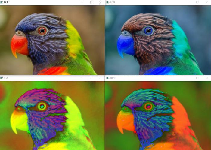
For color images, we typically calculate a histogram for each channel (B, G, R) to analyze the color distribution.

Code Example

import cv2
import numpy as np
import matplotlib.pyplot as plt
# 1. Read a color image
image = cv2.imread('path/to/your/color_image.jpg')
# OpenCV reads images in BGR format by default
if image is None:
    print("Error: Could not read the image.")
    exit()
# 2. Calculate histograms for each color channel
# We calculate the histogram for the Blue, Green, and Red channels
hist_b = cv2.calcHist([image], [0], None, [256], [0, 256]) # Blue channel
hist_g = cv2.calcHist([image], [1], None, [256], [0, 256]) # Green channel
hist_r = cv2.calcHist([image], [2], None, [256], [0, 256]) # Red channel
# 3. Display the image and its histograms
plt.figure(figsize=(15, 6))
# Plot the image (convert BGR to RGB for correct color display with matplotlib)
plt.subplot(121), plt.imshow(cv2.cvtColor(image, cv2.COLOR_BGR2RGB))'Color Image'), plt.xticks([]), plt.yticks([])
# Plot the histograms
plt.subplot(122)
plt.plot(hist_b, color='b', label='Blue Channel')
plt.plot(hist_g, color='g', label='Green Channel')
plt.plot(hist_r, color='r', label='Red Channel')'Color Histogram')
plt.xlabel('Pixel Intensity')
plt.ylabel('Pixel Count')
plt.xlim([0, 256])
plt.legend()
plt.show()

Explanation

• When reading a color image, OpenCV loads it in BGR (Blue, Green, Red) order.
• To get the histogram for the Blue channel, we use [0], for Green [1], and for Red [2].
• We plot all three histograms on the same graph with different colors for easy comparison.

Using a Mask

A mask allows you to calculate the histogram for a specific region of interest (ROI) in the image. The mask must be an 8-bit single-channel array with the same dimensions as the image, where non-zero pixels are the region of interest.

Code Example

import cv2
import numpy as np
import matplotlib.pyplot as plt
# 1. Read an image
image = cv2.imread('path/to/your/image.jpg', cv2.IMREAD_GRAYSCALE)
if image is None:
    print("Error: Could not read the image.")
    exit()
# 2. Create a mask
# Let's create a circular mask in the center of the image
height, width = image.shape
center = (width // 2, height // 2)
radius = min(width, height) // 4
# Create a black mask with the same size as the image
mask = np.zeros(image.shape[:2], np.uint8)
# Draw a white circle on the mask
cv2.circle(mask, center, radius, 255, -1) # -1 for filled circle
# 3. Calculate histogram for the full image and the masked region
hist_full = cv2.calcHist([image], [0], None, [256], [0, 256])
hist_masked = cv2.calcHist([image], [0], mask, [256], [0, 256])
# 4. Display results
plt.figure(figsize=(12, 8))
# Original image
plt.subplot(221), plt.imshow(image, cmap='gray')'Original Image'), plt.xticks([]), plt.yticks([])
# Mask
plt.subplot(222), plt.imshow(mask, cmap='gray')'Mask'), plt.xticks([]), plt.yticks([])
# Histogram of full image
plt.subplot(223), plt.plot(hist_full)'Full Image Histogram')
plt.xlim([0, 256])
# Histogram of masked region
plt.subplot(224), plt.plot(hist_masked)'Masked Region Histogram')
plt.xlim([0, 256])
plt.tight_layout()
plt.show()

Explanation

• We create a mask array of zeros.
• cv2.circle() is used to draw a filled white circle on the mask. This white area defines our ROI.
• When we pass this mask to cv2.calcHist(), the function only counts pixels from the original image where the mask has a non-zero value.

Histogram Equalization

Histogram equalization is a method to improve the contrast of an image by "stretching out" the intensity range. It works by transforming the image so that its histogram is as flat as possible. This is extremely useful for images with low contrast.

How it works:

1. Calculate the image's histogram.
2. Calculate the Cumulative Distribution Function (CDF).
3. Use the CDF to create a lookup table to map the old pixel values to new ones.

Code Example (Grayscale)

import cv2
import numpy as np
import matplotlib.pyplot as plt
# 1. Read a low-contrast grayscale image
image = cv2.imread('path/to/your/low_contrast_image.jpg', cv2.IMREAD_GRAYSCALE)
if image is None:
    print("Error: Could not read the image.")
    exit()
# 2. Apply Histogram Equalization
equalized_image = cv2.equalizeHist(image)
# 3. Calculate histograms for comparison
hist_original = cv2.calcHist([image], [0], None, [256], [0, 256])
hist_equalized = cv2.calcHist([equalized_image], [0], None, [256], [0, 256])
# 4. Display results
plt.figure(figsize=(15, 10))
# Original Image and Histogram
plt.subplot(221), plt.imshow(image, cmap='gray')'Original Image'), plt.xticks([]), plt.yticks([])
plt.subplot(222), plt.plot(hist_original)'Original Histogram')
plt.xlim([0, 256])
# Equalized Image and Histogram
plt.subplot(223), plt.imshow(equalized_image, cmap='gray')'Equalized Image'), plt.xticks([]), plt.yticks([])
plt.subplot(224), plt.plot(hist_equalized)'Equalized Histogram')
plt.xlim([0, 256])
plt.tight_layout()
plt.show()

Explanation

• cv2.equalizeHist() is a single, powerful function that performs the entire process.
• Notice how the histogram of the equalized image is much wider and flatter, indicating better use of the available intensity range and thus higher contrast.

Histogram Equalization for Color Images

You should not apply cv2.equalizeHist() directly to a color image. Doing so would distort the colors because it operates on each channel independently. The correct approach is to:

1. Convert the image to the YCrCb color space (Luminance, Chrominance Red, Chrominance Blue).
2. Equalize only the Luminance (Y) channel.
3. Convert the image back to the BGR color space.

import cv2
import numpy as np
import matplotlib.pyplot as plt
# 1. Read a color image
image = cv2.imread('path/to/your/low_contrast_color_image.jpg')
if image is None:
    print("Error: Could not read the image.")
    exit()
# 2. Convert to YCrCb color space
ycrcb_image = cv2.cvtColor(image, cv2.COLOR_BGR2YCrCb)
# 3. Split the channels
y, cr, cb = cv2.split(ycrcb_image)
# 4. Equalize the Y channel (Luminance)
y_equalized = cv2.equalizeHist(y)
# 5. Merge the channels back
equalized_ycrcb = cv2.merge([y_equalized, cr, cb])
# 6. Convert back to BGR color space
equalized_bgr = cv2.cvtColor(equalized_ycrcb, cv2.COLOR_YCrCb2BGR)
# 7. Display the results
plt.figure(figsize=(12, 6))
plt.subplot(121), plt.imshow(cv2.cvtColor(image, cv2.COLOR_BGR2RGB))'Original Color Image'), plt.xticks([]), plt.yticks([])
plt.subplot(122), plt.imshow(cv2.cvtColor(equalized_bgr, cv2.COLOR_BGR2RGB))'Equalized Color Image'), plt.xticks([]), plt.yticks([])
plt.show()

Summary of Key Functions