Of course! Here is a comprehensive guide on how to use Support Vector Machines (SVMs) with Python's scikit-learn library. We'll cover the core concepts, different types of SVMs, a step-by-step code example, and important parameters.
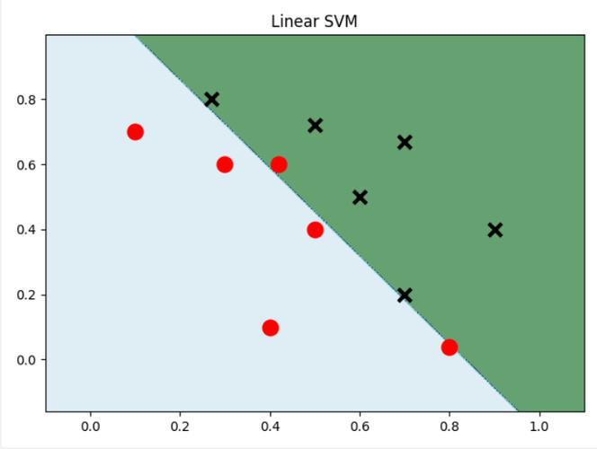
What is a Support Vector Machine (SVM)?
An SVM is a powerful and versatile supervised machine learning algorithm used for both classification and regression. The core idea is to find an optimal hyperplane that best separates the data points of different classes.
- For Classification: The goal is to find a hyperplane (a line in 2D, a plane in 3D, or a manifold in higher dimensions) that creates the widest possible "street" or margin between the classes of data points. The data points that lie closest to this hyperplane are called Support Vectors. They are the critical elements that define the position and orientation of the hyperplane.
- For Regression: Instead of finding a separating hyperplane, SVMs find a function that deviates from the actual target values by a value no greater than a specified margin, while at the same time being as "flat" as possible.
Types of SVMs in Scikit-learn
Scikit-learn provides different SVM implementations, each suited for a specific task.
| Algorithm | Class Name | Use Case | Kernel Trick |
|---|---|---|---|
| Linear SVM | sklearn.svm.SVC |
For linearly separable data. Fast and efficient. | No (uses a linear kernel) |
| Non-Linear SVM | sklearn.svm.SVC |
For data that is not linearly separable. | Yes (e.g., RBF, Polynomial) |
| Linear SVM (Regression) | sklearn.svm.SVR |
For linear regression tasks. | No (uses a linear kernel) |
| Non-Linear SVM (Regression) | sklearn.svm.SVR |
For non-linear regression tasks. | Yes (e.g., RBF, Polynomial) |
SVCstands for Support Vector Classification.SVRstands for Support Vector Regression.
We will focus on SVC for classification in this guide.
The Kernel Trick
The real power of SVMs comes from the kernel trick. It allows the algorithm to learn non-linear boundaries by implicitly mapping the input features into a higher-dimensional space where a linear separation is possible.
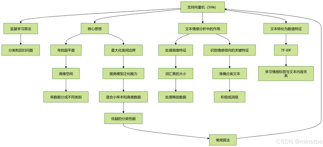
Common kernels in scikit-learn:
linear:(X @ X.T + c)poly:(gamma * X @ X.T + coef0)^degreerbf(Radial Basis Function):exp(-gamma * ||X - X'||^2)- This is the most popular kernel.sigmoid:tanh(gamma * X @ X.T + coef0)
Step-by-Step SVM Classification Example with Scikit-learn
Let's build a complete example to classify data points into two classes.
Step 1: Import Necessary Libraries
import numpy as np
import matplotlib.pyplot as plt
from sklearn import datasets
from sklearn.model_selection import train_test_split
from sklearn.svm import SVC
from sklearn.metrics import accuracy_score, classification_report, confusion_matrix
Step 2: Load and Prepare the Data
We'll use the famous Iris dataset, which is conveniently available in scikit-learn. For simplicity, we'll only use two features (sepal length and sepal width) and two classes (setosa and versicolor) so we can easily visualize the results.
# Load the iris dataset
iris = datasets.load_iris()
X = iris.data
y = iris.target
# For simplicity, we'll use only the first two features and the first two classes
# (setosa and versicolor)
X = X[y != 2]  # Remove class '2' (virginica)
y = y[y != 2]
# Split the data into training and testing sets
X_train, X_test, y_train, y_test = train_test_split(
    X, y, test_size=0.3, random_state=42
)
print(f"Training data shape: {X_train.shape}")
print(f"Testing data shape: {X_test.shape}")
Step 3: Create and Train the SVM Model
We'll start with a Linear SVM. The C parameter is a regularization parameter. It controls the trade-off between achieving a wide margin and minimizing the classification error.
- Small
C: A wider margin, but may misclassify some training points (soft margin). - Large
C: A narrower margin, tries to classify all training points correctly (hard margin).
# Create an SVM classifier with a linear kernel
# C is the regularization parameter
svm_classifier = SVC(kernel='linear', C=1.0, random_state=42)
# Train the model on the training data
svm_classifier.fit(X_train, y_train)
Step 4: Make Predictions
Now, we use the trained model to predict the classes for the test set.
# Make predictions on the test data
y_pred = svm_classifier.predict(X_test)
Step 5: Evaluate the Model
Let's check how well our model performed.
# Calculate accuracy
accuracy = accuracy_score(y_test, y_pred)
print(f"Accuracy: {accuracy:.2f}")
# Display a detailed classification report
print("\nClassification Report:")
print(classification_report(y_test, y_pred, target_names=iris.target_names[:2]))
# Display the confusion matrix
print("\nConfusion Matrix:")
print(confusion_matrix(y_test, y_pred))
Step 6: Visualize the Results (for 2D data)
Since we are using only two features, we can plot the decision boundary and the support vectors.
def plot_decision_boundary(X, y, model):
    # Create a mesh to plot the decision boundary
    x_min, x_max = X[:, 0].min() - 1, X[:, 0].max() + 1
    y_min, y_max = X[:, 1].min() - 1, X[:, 1].max() + 1
    xx, yy = np.meshgrid(np.arange(x_min, x_max, 0.02),
                         np.arange(y_min, y_max, 0.02))
    # Predict the class for each point in the mesh
    Z = model.predict(np.c_[xx.ravel(), yy.ravel()])
    Z = Z.reshape(xx.shape)
    # Plot the decision boundary and the margins
    plt.contourf(xx, yy, Z, alpha=0.3)
    # Plot the training points
    plt.scatter(X[:, 0], X[:, 1], c=y, edgecolors='k', s=50, cmap=plt.cm.coolwarm)
    # Highlight the support vectors
    plt.scatter(model.support_vectors_[:, 0], model.support_vectors_[:, 1],
                s=100, facecolors='none', edgecolors='k', linewidth=2)
    plt.title("SVM with Linear Kernel")
    plt.xlabel("Sepal length")
    plt.ylabel("Sepal width")
    plt.show()
# Plot the decision boundary
plot_decision_boundary(X_train, y_train, svm_classifier)
This plot will show the data points, the decision boundary, and the support vectors (circled points).
Using a Non-Linear Kernel (RBF)
Now, let's see what happens when we use a non-linear dataset and an RBF kernel. We'll generate a synthetic dataset using make_moons.
Step 1: Generate Non-Linear Data
from sklearn.datasets import make_moons
# Generate a non-linear dataset
X_moons, y_moons = make_moons(n_samples=200, noise=0.2, random_state=42)
# Split the data
X_train_m, X_test_m, y_train_m, y_test_m = train_test_split(
    X_moons, y_moons, test_size=0.3, random_state=42
)
Step 2: Train the SVM with RBF Kernel
For the RBF kernel, two important parameters are:
C: Regularization parameter.gamma: Kernel coefficient. It defines how far the influence of a single training example reaches.- Small
gamma: A large similarity radius (points far away are considered similar). - Large
gamma: A small similarity radius (only close points are considered similar).
- Small
# Create an SVM classifier with an RBF kernel
# C and gamma are important parameters to tune
svm_rbf = SVC(kernel='rbf', C=1.0, gamma='scale', random_state=42)
# Train the model
svm_rbf.fit(X_train_m, y_train_m)
Step 3: Evaluate and Visualize
# Make predictions and evaluate
y_pred_m = svm_rbf.predict(X_test_m)
print(f"Accuracy (RBF Kernel): {accuracy_score(y_test_m, y_pred_m):.2f}")
# Visualize the results
plot_decision_boundary(X_train_m, y_train_m, svm_rbf)
You will see that the RBF kernel creates a highly non-linear, curved decision boundary that successfully separates the two moon-shaped clusters.
Summary of Key Parameters
| Parameter | Description | Typical Tuning Strategy |
|---|---|---|
kernel |
Specifies the kernel type to be used in the algorithm. | 'linear', 'poly', 'rbf', 'sigmoid'. 'rbf' is a good default. |
C |
Regularization parameter. | A small C creates a smoother decision boundary. A large C tries to classify all points correctly. Use GridSearchCV to find the best value. |
gamma |
Kernel coefficient for 'rbf', 'poly', and 'sigmoid'. |
'scale' is often a good default (1 / (n_features * X.var())). 'auto' is another option (1 / n_features). If gamma is too large, the model may overfit. |
degree |
Degree of the polynomial kernel function ('poly'). |
Ignored by other kernels. Typically small integers (2, 3, 4). |
Practical Tips
-
Feature Scaling: SVMs are sensitive to the scale of the features. Always scale your data (e.g., using
StandardScalerorMinMaxScaler) before training an SVM model.from sklearn.preprocessing import StandardScaler scaler = StandardScaler() X_train_scaled = scaler.fit_transform(X_train) X_test_scaled = scaler.transform(X_test)
-
Parameter Tuning: The performance of an SVM is highly dependent on
Candgamma. UseGridSearchCVorRandomizedSearchCVto find the optimal combination of hyperparameters.from sklearn.model_selection import GridSearchCV param_grid = { 'C': [0.1, 1, 10, 100], 'gamma': ['scale', 'auto', 0.1, 1, 10], 'kernel': ['rbf'] } grid_search = GridSearchCV(SVC(), param_grid, refit=True, verbose=2, cv=5) grid_search.fit(X_train_scaled, y_train) print(f"Best parameters: {grid_search.best_params_}") best_svm = grid_search.best_estimator_

