Of course! Here is a comprehensive guide to image skeletonization in Python, covering the concept, different methods, and practical code examples using popular libraries.
What is Skeletonization?
Skeletonization (or topological thinning) is a process of reducing a binary shape to its "skeleton" or "medial axis." The skeleton is a set of pixels that represents the centerline or core structure of the shape. It's a one-pixel-wide representation that preserves the topology (connectivity) of the original shape.
Common Applications:
- Character Recognition (OCR): Simplifying characters for easier classification.
- Fingerprint Recognition: Extracting unique ridge patterns.
- Medical Imaging: Analyzing blood vessels or neural pathways.
- Shape Analysis and Recognition: Creating a canonical representation of a shape for comparison.
Prerequisites
You'll need a few Python libraries. If you don't have them, install them using pip:
pip install numpy opencv-python scikit-image matplotlib
- NumPy: For efficient array manipulation.
- OpenCV (
cv2): For image loading, preprocessing, and some skeletonization algorithms. - scikit-image (
skimage): Contains powerful and easy-to-use skeletonization functions. - Matplotlib: For displaying the images.
Method 1: Using scikit-image (Recommended)
The skimage.morphology module provides a robust and widely-used thinning algorithm. It's often the best place to start.
Algorithm: Zhang-Suen Thinning
This is a classic iterative thinning algorithm that works by repeatedly stripping pixels from the boundary of the shape based on a set of conditions.
Code Example
import cv2
import numpy as np
from skimage.morphology import skeletonize
from skimage.util import invert
import matplotlib.pyplot as plt
# 1. Load the image and convert to grayscale
# We'll use a simple rectangle for demonstration
image = np.zeros((256, 256), dtype=np.uint8)
cv2.rectangle(image, (50, 50), (200, 200), 255, -1) # -1 for filled rectangle
# For skeletonize, the image must be binary (0 or 1) and the object should be "True" (1).
# The algorithm works on the foreground (white pixels). If your object is black,
# you need to invert it.
binary_image = image > 0 # This creates a boolean array (True for object, False for background)
# 2. Perform skeletonization
skeleton = skeletonize(binary_image)
# 3. Display the results
fig, axes = plt.subplots(1, 2, figsize=(10, 5))
ax = axes.ravel()
ax[0].imshow(image, cmap='gray')
ax[0].set_title('Original Binary Image')
ax[0].axis('off')
# The skeleton is a boolean array, so we convert it to uint8 for display
ax[1].imshow(skeleton.astype(np.uint8) * 255, cmap='gray')
ax[1].set_title('Skeleton (Zhang-Suen)')
ax[1].axis('off')
plt.tight_layout()
plt.show()
Output:
Method 2: Using OpenCV (cv2.ximgproc.thinning)
OpenCV also has a thinning function, but it's part of the ximgproc module, which needs to be explicitly loaded. This function is highly optimized and can be faster than the scikit-image implementation for large images.
Code Example
import cv2
import numpy as np
import matplotlib.pyplot as plt
# 1. Load the image and convert to grayscale
image = np.zeros((256, 256), dtype=np.uint8)
cv2.rectangle(image, (50, 50), (200, 200), 255, -1)
# 2. Perform skeletonization using OpenCV
# The image must be 8-bit single-channel (binary).
# The thinningType can be THINNING_ZHANGSUEN or THINNING_GUOHALL
skeleton = cv2.ximgproc.thinning(image, cv2.ximgproc.THINNING_ZHANGSUEN)
# 3. Display the results
fig, axes = plt.subplots(1, 2, figsize=(10, 5))
ax = axes.ravel()
ax[0].imshow(image, cmap='gray')
ax[0].set_title('Original Binary Image')
ax[0].axis('off')
ax[1].imshow(skeleton, cmap='gray')
ax[1].set_title('Skeleton (OpenCV Zhang-Suen)')
ax[1].axis('off')
plt.tight_layout()
plt.show()
Note: If you get an error like module 'cv2' has no attribute 'ximgproc', it means your OpenCV build was not compiled with the ximgproc module. You may need to recompile OpenCV or use a pre-built package that includes it (like the one from conda-forge).
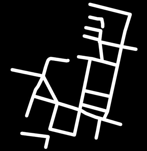
Method 3: Using Morphological Operations (Manual Approach)
This method gives you more control and helps you understand the underlying process. The idea is to use an erosion operation, but with a special structuring element that preserves connectivity.
The most common structuring element for this is the "cross" (or "plus") shape.
Algorithm: Medial Axis Transform (MAT)
- Distance Transform: First, compute the distance transform of the binary image. This gives each pixel a value representing its distance to the nearest background pixel. The "ridge" of this distance map corresponds to the medial axis.
- Local Maxima: Find the local maxima in the distance map. These pixels form the skeleton.
Code Example
import cv2
import numpy as np
import matplotlib.pyplot as plt
# 1. Load the image and convert to binary
image = np.zeros((256, 256), dtype=np.uint8)
cv2.rectangle(image, (50, 50), (200, 200), 255, -1)
cv2.circle(image, (100, 100), 30, 255, -1)
# 2. Compute the distance transform
# The output is a floating-point image where pixel values are distances.
dist_transform = cv2.distanceTransform(image, cv2.DIST_L2, 3)
# 3. Find the local maxima of the distance transform
# We can do this by thresholding the distance transform at a certain percentage
# of its maximum value.
_, skeleton = cv2.threshold(dist_transform, 0.7 * dist_transform.max(), 255, 0)
skeleton = np.uint8(skeleton)
# 4. Display the results
fig, axes = plt.subplots(1, 3, figsize=(15, 5))
ax = axes.ravel()
ax[0].imshow(image, cmap='gray')
ax[0].set_title('Original Binary Image')
ax[0].axis('off')
ax[1].imshow(dist_transform, cmap='jet') # Use a colormap to see the distance values
ax[1].set_title('Distance Transform')
ax[1].axis('off')
ax[2].imshow(skeleton, cmap='gray')
ax[2].set_title('Skeleton (from Distance Transform)')
ax[2].axis('off')
plt.tight_layout()
plt.show()
Output:
Important Considerations and Preprocessing
Skeletonization is sensitive to the quality of the input binary image. You often need to preprocess your images.
-
Thresholding: Your image must be binary. If you start from a grayscale image, you need to binarize it using a threshold (e.g., Otsu's thresholding).
# Example: Otsu's thresholding
_, binary_image = cv2.threshold(grayscale_image, 0, 255, cv2.THRESH_BINARY + cv2.THRESH_OTSU)
-
Noise: Small noise or speckles can turn into unwanted branches in the skeleton. It's crucial to clean the image.
# Example: Remove small noise using morphological opening
kernel = np.ones((3,3), np.uint8)
cleaned_image = cv2.morphologyEx(binary_image, cv2.MORPH_OPEN, kernel)
-
Holes: If your shape has holes, the skeletonization algorithm might produce artifacts or break connectivity. You may need to fill holes before processing.
# Example: Fill holes
contours, _ = cv2.findContours(binary_image, cv2.RETR_EXTERNAL, cv2.CHAIN_APPROX_SIMPLE)
filled_image = np.zeros_like(binary_image)
cv2.drawContours(filled_image, contours, -1, 255, -1)
Summary of Methods
| Method | Library | Pros | Cons | Best For |
|---|---|---|---|---|
| Zhang-Suen / Guo-Hall | scikit-image |
Easy to use, robust, good results. | Can be slower for very large images. | General purpose, quick implementation. |
| Thinning | OpenCV (ximgproc) |
Highly optimized, fast. | Requires a specific OpenCV build. | Performance-critical applications. |
| Medial Axis Transform | OpenCV |
More intuitive (distance-based), preserves shape thickness info. | Can be less "clean" than thinning, sensitive to noise. | Understanding the concept, applications where thickness matters. |
For most users, starting with skimage.morphology.skeletonize is the recommended approach due to its simplicity and reliability.



![Python reversed()怎么用?[::-1]和它有啥区别?](https://www.jerry.net.cn/zb_users/cache/thumbs/ed28fc61e3e820b31c4e5ed7c6a8b7fc-252-157-1.jpeg)

