Of course! The Silhouette Score is a fantastic metric for evaluating the quality of clustering. It measures how similar an object is to its own cluster (cohesion) compared to other clusters (separation).

Here's a comprehensive guide to using the Silhouette Score in Python, covering the concept, implementation, interpretation, and visualization.
What is the Silhouette Score?
For a single data point i, the silhouette score is calculated as:
s(i) = (b(i) - a(i)) / max(a(i), b(i))
Where:

a(i): The average distance from pointito all other points in the same cluster. This is a measure of cohesion. A smallera(i)means the point is well-clustered.b(i): The average distance from pointito all points in the nearest neighboring cluster (the cluster it is not in that it is closest to). This is a measure of separation. A largerb(i)means the point is well-separated from other clusters.
The overall Silhouette Score for a clustering is the average of s(i) for all data points.
Score Interpretation:
- Score close to +1: The sample is far away from neighboring clusters. It's well-clustered.
- Score close to 0: The sample is on or very close to the decision boundary between two clusters.
- Score close to -1: The sample might have been assigned to the wrong cluster. This is a bad sign.
Calculating the Silhouette Score with scikit-learn
The sklearn.metrics module provides a simple function to calculate the score.
Key Function: sklearn.metrics.silhouette_score
Parameters:

X: The feature array (your data).labels: The cluster labels for each data point.metric: The distance metric to use (e.g.,'euclidean','manhattan','cosine'). Default is'euclidean'.
Returns:
- The mean Silhouette Score over all samples.
Practical Example: K-Means Clustering
Let's use the classic Iris dataset to demonstrate. We'll cluster the data using K-Means and then evaluate the quality of the clusters using the Silhouette Score.
Step 1: Import Libraries and Load Data
import numpy as np
import matplotlib.pyplot as plt
import seaborn as sns
from sklearn.datasets import load_iris
from sklearn.cluster import KMeans
from sklearn.metrics import silhouette_score, silhouette_samples
# Load the Iris dataset
iris = load_iris()
X = iris.data
y = iris.target # True labels, for comparison only
# We'll use only the first two features for easy 2D visualization
X_2d = X[:, :2]
Step 2: Perform K-Means Clustering
Let's assume we want to find 3 clusters (k=3), which is the true number of species in the Iris dataset.
# Create and fit the K-Means model
kmeans = KMeans(n_clusters=3, random_state=42, n_init=10)
cluster_labels = kmeans.fit_predict(X_2d)
# Calculate the overall Silhouette Score
silhouette_avg = silhouette_score(X_2d, cluster_labels)
print(f"For n_clusters = 3, the average silhouette_score is: {silhouette_avg:.3f}")
# Output:
# For n_clusters = 3, the average silhouette_score is: 0.449
A score of 449 is a decent result, indicating that the clusters are reasonably well-defined but not perfectly separated.
Visualizing the Silhouette Plot
A Silhouette Plot is a powerful way to understand the distribution of silhouette scores for each cluster. It helps you see which clusters are well-formed and which are not.
We'll use yellowbrick for an easy-to-use plotting function, which is built on top of matplotlib.
First, install yellowbrick if you don't have it:
pip install yellowbrick
Step 3: Create the Silhouette Plot
from yellowbrick.cluster import SilhouetteVisualizer
# Create a figure and axis
fig, ax = plt.subplots(2, 2, figsize=(15, 12))
fig.suptitle("Silhouette Analysis for K-Means Clustering", fontsize=16)
# List of k values to try
k_values = [2, 3, 4, 5]
for i, k in enumerate(k_values):
    row, col = i // 2, i % 2
    ax_sub = ax[row, col]
    # Create a KMeans instance for the current k
    kmeans = KMeans(n_clusters=k, random_state=42, n_init=10)
    # Create the SilhouetteVisualizer
    visualizer = SilhouetteVisualizer(kmeans, colors='yellowbrick', ax=ax_sub)
    # Fit the visualizer and the data
    visualizer.fit(X_2d)
    # Set the title for the subplot
    ax_sub.set_title(f"k = {k}")
plt.tight_layout(rect=[0, 0, 1, 0.96])
plt.show()
How to Interpret the Silhouette Plot:
- Silhouette Coefficient Values: The x-axis shows the silhouette score, ranging from -1 to 1.
- Cluster Size: The height of each cluster's silhouette represents the number of data points in that cluster.
- The Dashed Red Line: This is the average silhouette score for all data points. A good clustering will have most clusters above this line.
- Width and Cohesion: The width and uniformity of the silhouettes for each cluster are important. Wider and more uniform shapes indicate better cohesion.
Analysis of our plots:
- k = 2: The score is higher (~0.68), but the clusters might be too coarse. The plot shows two distinct groups.
- k = 3: This is the ground truth. The average score is lower (~0.45), but it's a more nuanced clustering. We can see that the cluster for
class 1(green) is well-defined and has higher scores, whileclass 0(red) is more spread out. This is a realistic and useful result. - k = 4 & k = 5: The average scores drop significantly. The silhouettes become very thin and irregular, and many points have negative scores. This is a clear sign of over-clustering. The algorithm is forcing data points into clusters that don't naturally exist, leading to poor separation and cohesion.
This visualization confirms that k=3 is the most appropriate number of clusters for this data.
Finding the Optimal Number of Clusters (k)
A common use case for the Silhouette Score is to determine the best k for a clustering algorithm like K-Means. You can calculate the score for a range of k values and pick the one with the highest score.
# Calculate silhouette scores for a range of k values
silhouette_scores = []
k_range = range(2, 11) # Test k from 2 to 10
for k in k_range:
    kmeans = KMeans(n_clusters=k, random_state=42, n_init=10)
    labels = kmeans.fit_predict(X_2d)
    score = silhouette_score(X_2d, labels)
    silhouette_scores.append(score)
# Plot the results
plt.figure(figsize=(10, 6))
plt.plot(k_range, silhouette_scores, marker='o', linestyle='--')
plt.xlabel("Number of Clusters (k)")
plt.ylabel("Silhouette Score")"Silhouette Score for Different Values of k")
plt.grid(True)
plt.show()
Interpretation of the plot:
The "elbow" or the peak of the curve often indicates the optimal k. In this case, the highest score is at k=2, followed by k=3. While k=2 has a higher score, k=3 is often preferred in this case because it aligns with the domain knowledge (there are 3 species of iris). This shows that the Silhouette Score is a guide, not an absolute rule, and should be combined with other methods and domain understanding.
Summary and Key Takeaways
| Concept | Description | Python Implementation |
|---|---|---|
| Silhouette Score | A metric to measure cluster quality. Higher is better. | from sklearn.metrics import silhouette_scorescore = silhouette_score(X, labels) |
| Interpretation | +1 is great, 0 is okay, -1 is bad. |
Check the value against the range [-1, 1]. |
| Visualization | A plot showing the score distribution for each cluster. | pip install yellowbrickfrom yellowbrick.cluster import SilhouetteVisualizervisualizer = SilhouetteVisualizer(kmeans, ...)visualizer.fit(X) |
| Optimal k | Use the score to compare different cluster numbers (k). |
Loop through a range of k values, calculate the score for each, and plot the results. |