Of course! Let's dive deep into using Gradient Boosting Decision Trees (GBDT) with Python's scikit-learn library.

This guide will cover:

1. What is GBDT? (A brief, intuitive explanation)
2. Key sklearn Classes: GradientBoostingRegressor and GradientBoostingClassifier.
3. A Complete Step-by-Step Example: From data loading to prediction.
4. Hyperparameter Tuning: The most critical part of getting good results.
5. Pros and Cons: When to use (and not use) GBDT.
6. The Modern Alternative: HistGradientBoostingRegressor/Classifier.

What is GBDT? (Intuitive Explanation)

Imagine you're trying to solve a complex problem, like predicting house prices.

• Decision Tree (DT): A single decision tree is like asking one expert. This expert might look at the square footage and give a price estimate. It's simple but can be inaccurate and prone to mistakes (overfitting).

• Random Forest (Bagging): This is like asking a committee of 100 experts. Each expert looks at a random subset of features and data points. They all vote on the final price. This is much more robust and less prone to individual mistakes.

  
  （图片来源网络，侵删）

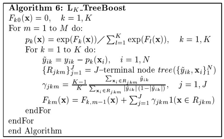
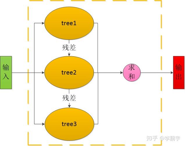
• Gradient Boosting (Boosting): This is a different approach. Instead of a committee of independent experts, it's like a team of experts where each subsequent expert's job is to correct the mistakes of the previous ones.

  1. Expert 1 makes a rough initial prediction (e.g., "$200,000").
  2. We calculate the errors (the difference between the prediction and the actual price).
  3. Expert 2 is trained specifically to predict these errors. If Expert 1 consistently underpriced large houses, Expert 2 will learn to add more value for them.
  4. The final prediction is Expert 1's prediction + Expert 2's prediction.
  5. We repeat this process, adding more "experts" (trees) that focus on the remaining errors of the combined team so far.

The "Gradient" part refers to how the algorithm finds the best way to correct the errors—it uses gradient descent to minimize the loss function (e.g., Mean Squared Error for regression).

Key sklearn Classes

Scikit-learn provides two main classes for GBDT:

• sklearn.ensemble.GradientBoostingRegressor: For regression problems (predicting a continuous value).
• sklearn.ensemble.GradientBoostingClassifier: For classification problems (predicting a category).

They share a very similar set of parameters.

Complete Step-by-Step Example (Regression)

Let's build a GBDT model to predict the California housing prices.

Step 1: Import Libraries

import numpy as np
import pandas as pd
from sklearn.model_selection import train_test_split
from sklearn.ensemble import GradientBoostingRegressor
from sklearn.metrics import mean_squared_error, r2_score
from sklearn.datasets import fetch_california_housing

Step 2: Load and Prepare Data

# Load the dataset
california = fetch_california_housing()
X = california.data
y = california.target
# For reproducibility, let's use a fixed random state
X_train, X_test, y_train, y_test = train_test_split(X, y, test_size=0.2, random_state=42)
print(f"Training set shape: {X_train.shape}")
print(f"Test set shape: {X_test.shape}")

Step 3: Initialize and Train the Model

This is where we set the key hyperparameters.

# Initialize the Gradient Boosting Regressor
# Let's start with some sensible defaults
gbr = GradientBoostingRegressor(
    n_estimators=100,      # Number of boosting stages (trees)
    learning_rate=0.1,     # Shrinkage factor
    max_depth=3,           # Maximum depth of the individual trees
    random_state=42
)
# Train the model
gbr.fit(X_train, y_train)
print("\nModel training complete.")

Step 4: Make Predictions and Evaluate

# Make predictions on the test set
y_pred = gbr.predict(X_test)
# Evaluate the model
mse = mean_squared_error(y_test, y_pred)
rmse = np.sqrt(mse)
r2 = r2_score(y_test, y_pred)
print(f"\n--- Model Evaluation ---")
print(f"Mean Squared Error (MSE): {mse:.4f}")
print(f"Root Mean Squared Error (RMSE): {rmse:.4f}")
print(f"R-squared (R²): {r2:.4f}")

Step 5: Feature Importance

A great feature of tree-based models is that they can tell you which features were most important for making predictions.

# Get feature importances
importances = gbr.feature_importances_
feature_names = california.feature_names
# Create a DataFrame for better visualization
feature_importance_df = pd.DataFrame({'feature': feature_names, 'importance': importances})
feature_importance_df = feature_importance_df.sort_values(by='importance', ascending=False)
print("\n--- Feature Importances ---")
print(feature_importance_df)

Hyperparameter Tuning (Crucial!)

The performance of GBDT is extremely sensitive to its hyperparameters. Here are the most important ones:

How to Tune? The best way is with GridSearchCV or RandomizedSearchCV from sklearn.model_selection.

from sklearn.model_selection import GridSearchCV
# Define the parameter grid to search
param_grid = {
    'n_estimators': [50, 100, 200],
    'learning_rate': [0.05, 0.1, 0.2],
    'max_depth': [3, 4, 5],
    'subsample': [0.8, 1.0]
}
# Initialize the base model
gbr_tune = GradientBoostingRegressor(random_state=42)
# Set up the GridSearchCV
# cv=3 means 3-fold cross-validation
# n_jobs=-1 uses all available CPU cores
grid_search = GridSearchCV(
    estimator=gbr_tune,
    param_grid=param_grid,
    cv=3,
    scoring='neg_mean_squared_error', # We want to minimize MSE
    n_jobs=-1,
    verbose=2 # Shows progress
)
# Fit the grid search to the data
grid_search.fit(X_train, y_train)
# Get the best parameters and the best score
print("\n--- Grid Search Results ---")
print(f"Best parameters found: {grid_search.best_params_}")
print(f"Best negative MSE score: {grid_search.best_score_:.4f}")
# Evaluate the best model on the test set
best_gbr = grid_search.best_estimator_
y_pred_best = best_gbr.predict(X_test)
rmse_best = np.sqrt(mean_squared_error(y_test, y_pred_best))
r2_best = r2_score(y_test, y_pred_best)
print(f"\n--- Best Model Evaluation on Test Set ---")
print(f"Best Model RMSE: {rmse_best:.4f}")
print(f"Best Model R²: {r2_best:.4f}")

Pros and Cons

Pros:

• High Predictive Accuracy: Often one of the best-performing models on tabular data.
• Flexibility: Can be used for both regression and classification.
• Feature Importance: Provides a clear measure of which features are most predictive.
• Handles Mixed Data Types: Works well with numerical and categorical features (after encoding).

Cons:

• Computationally Expensive: Training can be slow, especially with many trees and large datasets.
• Prone to Overfitting: If not tuned carefully (e.g., too many trees or too high a learning rate).
• Less Interpretable: A single decision tree is easy to visualize, but an ensemble of hundreds is a "black box".
• Sensitive to Hyperparameters: Performance heavily depends on good hyperparameter tuning.

The Modern Alternative: HistGradientBoosting

Scikit-learn has introduced a faster, more memory-efficient, and often more accurate version of GBDT called Histogram-based Gradient Boosting.

• How it works: Instead of finding the best split point among all unique values for a feature, it first bins (histograms) the feature values into discrete intervals. Then, it finds the best split among these bins. This is much faster.
• Advantages:
  • Speed: Training is significantly faster, especially on large datasets.
  • Memory: Uses less memory.
  • Performance: Often outperforms the classic GradientBoosting with default parameters.
  • Handles Missing Values: Can automatically handle missing values without imputation.

Example Usage:

from sklearn.ensemble import HistGradientBoostingRegressor
# Initialize the Hist Gradient Boosting Regressor
# Note: No 'n_estimators', uses 'max_iter' instead
hgb = HistGradientBoostingRegressor(
    max_iter=100,          # Number of boosting iterations (trees)
    learning_rate=0.1,
    max_depth=3,
    random_state=42
)
# Train and evaluate
hgb.fit(X_train, y_train)
y_pred_hgb = hgb.predict(X_test)
rmse_hgb = np.sqrt(mean_squared_error(y_test, y_pred_hgb))
r2_hgb = r2_score(y_test, y_pred_hgb)
print("\n--- HistGradientBoosting Evaluation ---")
print(f"HGB RMSE: {rmse_hgb:.4f}")
print(f"HGB R²: {r2_hgb:.4f}")

Recommendation: For most new projects, start with HistGradientBoostingRegressor or HistGradientBoostingClassifier. It's the modern, improved implementation of GBDT in scikit-learn. Only fall back to the classic GradientBoosting if you need exact reproducibility of older models or require a specific feature not present in the Hist version.