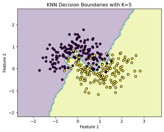
Of course! Here is a comprehensive guide to using the k-Nearest Neighbors (k-NN) algorithm in Python with the scikit-learn library.

We'll cover:
- What is k-NN? (A quick, intuitive explanation)
- The Workflow in
scikit-learn(The standard 4-step process) - A Complete, Runnable Code Example (Classification)
- Key Concepts & Important Considerations
- Choosing
k - Distance Metrics
- Feature Scaling
- Pros and Cons
- Choosing
- A Quick Look at k-NN for Regression
What is k-Nearest Neighbors (k-NN)?
k-NN is one of the simplest and most intuitive machine learning algorithms. It's a non-parametric, lazy learning algorithm.
-
Intuition: "Tell me who your neighbors are, and I'll tell you who you are."
-
How it works for Classification:
 (图片来源网络,侵删)
- When a new data point needs to be classified, the algorithm finds the
k"closest" data points from the training set. These are theknearest neighbors. - It then looks at the labels of these
kneighbors. - The algorithm assigns the most common label among the neighbors to the new data point.
- When a new data point needs to be classified, the algorithm finds the
-
Key Terms:
k(the parameter): The number of neighbors to consider. This is a hyperparameter you must choose.- "Nearest" (the distance): Closeness is measured using a distance metric, most commonly Euclidean distance.
The scikit-learn Workflow
Using any algorithm in scikit-learn generally follows these four steps:
- Import the necessary classes and functions.
- Instantiate the model (e.g.,
KNeighborsClassifier()). - Fit the model to your training data (
.fit()). - Predict on new, unseen data (
.predict()).
Complete Code Example (Classification)
Let's build a k-NN classifier to predict the species of an iris flower based on its sepal and petal measurements. This is a classic "Hello, World!" for machine learning.
# Step 1: Import necessary libraries
import numpy as np
import matplotlib.pyplot as plt
from sklearn.datasets import load_iris
from sklearn.model_selection import train_test_split
from sklearn.preprocessing import StandardScaler
from sklearn.neighbors import KNeighborsClassifier
from sklearn.metrics import accuracy_score, classification_report, confusion_matrix
# For better looking plots
import seaborn as sns
# Step 2: Load the dataset
# The Iris dataset is built into scikit-learn
iris = load_iris()
X = iris.data      # Features: sepal length, sepal width, petal length, petal width
y = iris.target    # Target: species of iris (0, 1, or 2)
# Let's see what the data looks like
print("Feature names:", iris.feature_names)
print("Target names:", iris.target_names)
print("\nFirst 5 rows of X:\n", X[:5])
print("\nFirst 5 rows of y:\n", y[:5])
# Step 3: Split data into training and testing sets
# We split the data to train the model on one subset and test its performance on another.
# test_size=0.3 means 30% of the data will be used for testing.
# random_state ensures reproducibility of the split.
X_train, X_test, y_train, y_test = train_test_split(X, y, test_size=0.3, random_state=42)
print(f"\nTraining set size: {X_train.shape[0]} samples")
print(f"Testing set size: {X_test.shape[0]} samples")
# --- VERY IMPORTANT: Feature Scaling ---
# k-NN is distance-based. Features with larger scales can dominate the distance calculation.
# We scale features to have a mean of 0 and a standard deviation of 1.
# We fit the scaler ONLY on the training data to avoid data leakage from the test set.
scaler = StandardScaler()
X_train_scaled = scaler.fit_transform(X_train)
X_test_scaled = scaler.transform(X_test) # Use the same scaler fitted on the training data
# Step 4: Instantiate the k-NN model
# Let's start with k=5. This is a common starting point.
k = 5
knn = KNeighborsClassifier(n_neighbors=k)
# Step 5: Fit the model to the scaled training data
knn.fit(X_train_scaled, y_train)
# Step 6: Make predictions on the scaled test data
y_pred = knn.predict(X_test_scaled)
# Step 7: Evaluate the model's performance
# Compare the predictions (y_pred) with the actual labels (y_test)
accuracy = accuracy_score(y_test, y_pred)
print(f"\nAccuracy with k={k}: {accuracy:.4f}")
# A more detailed report
print("\nClassification Report:")
print(classification_report(y_test, y_pred, target_names=iris.target_names))
# Visualize the confusion matrix
cm = confusion_matrix(y_test, y_pred)
plt.figure(figsize=(8, 6))
sns.heatmap(cm, annot=True, fmt='d', cmap='Blues', xticklabels=iris.target_names, yticklabels=iris.target_names)
plt.xlabel('Predicted Label')
plt.ylabel('True Label')'Confusion Matrix')
plt.show()
Key Concepts & Important Considerations
How to Choose the Best k?
The choice of k is critical and is determined through hyperparameter tuning. A common method is to test a range of k values and see which one performs best on the validation set.

- Small
k(e.g., k=1):- Pros: Can capture fine-grained patterns.
- Cons: Highly sensitive to noise and outliers. The model becomes too complex and may overfit the training data.
- Large
k:- Pros: Smoother decision boundaries, less sensitive to noise.
- Cons: May underfit the data by ignoring local structures. The model becomes too simple and might misclassify points near class boundaries.
Let's find the best k using a loop:
# We will use cross-validation for a more robust estimate of accuracy for each k.
from sklearn.model_selection import cross_val_score
# Try a range of k values
k_values = list(range(1, 31))
cv_scores = []
for k in k_values:
    knn = KNeighborsClassifier(n_neighbors=k)
    # Perform 5-fold cross-validation and get the mean accuracy
    scores = cross_val_score(knn, X_train_scaled, y_train, cv=5, scoring='accuracy')
    cv_scores.append(scores.mean())
# Find the k with the highest average accuracy
best_k_index = np.argmax(cv_scores)
best_k = k_values[best_k_index]
best_score = cv_scores[best_k_index]
print(f"Best k: {best_k}")
print(f"Best cross-validation accuracy: {best_score:.4f}")
# Plot the results to visualize the performance
plt.figure(figsize=(10, 6))
plt.plot(k_values, cv_scores, marker='o', linestyle='-', color='b')
plt.xlabel('Number of Neighbors (k)')
plt.ylabel('Cross-Validated Accuracy')'k-NN Varying Number of Neighbors')
plt.axvline(x=best_k, color='r', linestyle='--', label=f'Best k = {best_k}')
plt.legend()
plt.grid(True)
plt.show()
Feature Scaling is Crucial for k-NN
As mentioned earlier, k-NN relies on distance. If one feature (e.g., sepal length in cm, range 4-8) has a much larger scale than another (e.g., petal width in cm, range 0.1-2.5), the distance calculation will be almost entirely determined by the first feature.
- Solution: Always scale your features before using k-NN.
StandardScaleris a great choice, butMinMaxScaleris also common.
Pros and Cons of k-NN
| Pros | Cons |
|---|---|
| Simple to understand and implement. | Computationally expensive at prediction time. |
| No training phase (it's a "lazy" learner). | Needs to store the entire training dataset. |
| Versatile: Can be used for classification and regression. | Sensitive to irrelevant features. |
| Naturally multi-class. | Sensitive to the scale of the data. |
Sensitive to the choice of k and distance metric. |
k-NN for Regression
k-NN can also be used for regression. Instead of taking a "majority vote," it averages the values of the k nearest neighbors.
- How it works:
- Find the
knearest neighbors to the new data point. - The predicted value is the average (or weighted average) of the target values of these
kneighbors.
- Find the
Example:
from sklearn.neighbors import KNeighborsRegressor
from sklearn.datasets import load_boston # Note: load_boston is deprecated, but good for a quick example.
# For a modern example, you could use fetch_openml('boston-house-prices')
# Let's use a simple synthetic dataset for clarity
from sklearn.datasets import make_regression
X_reg, y_reg = make_regression(n_samples=100, n_features=1, noise=20, random_state=42)
X_train_reg, X_test_reg, y_train_reg, y_test_reg = train_test_split(X_reg, y_reg, test_size=0.3, random_state=42)
# Scale the features for regression as well
scaler_reg = StandardScaler()
X_train_reg_scaled = scaler_reg.fit_transform(X_train_reg)
X_test_reg_scaled = scaler_reg.transform(X_test_reg)
# Instantiate and fit the regressor
knn_reg = KNeighborsRegressor(n_neighbors=5)
knn_reg.fit(X_train_reg_scaled, y_train_reg)
# Predict
y_pred_reg = knn_reg.predict(X_test_reg_scaled)
# Evaluate
from sklearn.metrics import mean_squared_error, r2_score
mse = mean_squared_error(y_test_reg, y_pred_reg)
r2 = r2_score(y_test_reg, y_pred_reg)
print(f"\n--- k-NN Regression ---")
print(f"Mean Squared Error: {mse:.2f}")
print(f"R-squared: {r2:.2f}")
# Visualize the results
plt.figure(figsize=(10, 6))
plt.scatter(X_test_reg, y_test_reg, color='blue', label='Actual Data')
plt.scatter(X_test_reg, y_pred_reg, color='red', label='Predicted Data')
plt.xlabel('Feature')
plt.ylabel('Target Value')'k-NN Regression (k=5)')
plt.legend()
plt.show() 

