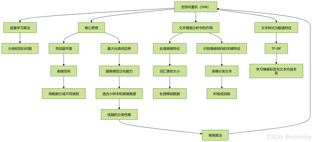
Of course! An "SVM problem" in Python can mean a few different things, ranging from a simple implementation to a more complex, real-world challenge. I'll cover the most common scenarios, starting with the basics and moving to more advanced topics.

Let's break it down into sections:

1. The Basic Problem: Implementing a Simple SVM (Using scikit-learn)
2. The Core Problem: Understanding the Math & Theory (The Optimization Problem)
3. The Real-World Problem: Hyperparameter Tuning & Evaluation
4. The Advanced Problem: Solving a Non-Linear Problem (The Kernel Trick)
5. The Final Problem: Putting It All Together in a Full Workflow

The Basic Problem: Implementing a Simple SVM

This is the most common task. You have some labeled data, and you want to train a Support Vector Machine to classify new data points.

The Scenario

We'll create a simple 2D dataset with two classes and use an SVM to find the optimal hyperplane that separates them.

Python Code (scikit-learn)

scikit-learn is the go-to library for machine learning in Python. Its SVC (Support Vector Classifier) class makes this incredibly easy.

import numpy as np
import matplotlib.pyplot as plt
from sklearn.svm import SVC
from sklearn.datasets import make_classification
from sklearn.model_selection import train_test_split
# --- 1. Generate Sample Data ---
# Let's create a 2D dataset with 2 classes
X, y = make_classification(
    n_samples=100,       # 100 data points
    n_features=2,        # 2 features (x1, x2)
    n_informative=2,     # Both features are useful
    n_redundant=0,       # No redundant features
    n_clusters_per_class=1,
    flip_y=0.05,         # Add a little noise
    random_state=42      # For reproducibility
)
# Split data into training and testing sets
X_train, X_test, y_train, y_test = train_test_split(X, y, test_size=0.3, random_state=42)
# --- 2. Create and Train the SVM Model ---
# We'll use a linear kernel for now.
# C is the regularization parameter. A smaller C creates a wider street (more margin violations).
model = SVC(kernel='linear', C=1.0, random_state=42)
# Train the model on our training data
model.fit(X_train, y_train)
# --- 3. Evaluate the Model ---
accuracy = model.score(X_test, y_test)
print(f"Model Accuracy: {accuracy:.2f}")
# --- 4. Visualize the Results ---
def plot_decision_boundary(X, y, model):
    # Create a grid of points to plot
    x_min, x_max = X[:, 0].min() - 1, X[:, 0].max() + 1
    y_min, y_max = X[:, 1].min() - 1, X[:, 1].max() + 1
    xx, yy = np.meshgrid(np.arange(x_min, x_max, 0.02),
                         np.arange(y_min, y_max, 0.02))
    # Predict the class for each point in the grid
    Z = model.predict(np.c_[xx.ravel(), yy.ravel()])
    Z = Z.reshape(xx.shape)
    # Plot the decision boundary and the data points
    plt.contourf(xx, yy, Z, alpha=0.3)
    plt.scatter(X[:, 0], X[:, 1], c=y, edgecolors='k')
    plt.title("SVM Decision Boundary")
    plt.xlabel("Feature 1")
    plt.ylabel("Feature 2")
    plt.show()
plot_decision_boundary(X, y, model)

Output:

Model Accuracy: 0.93

And a plot showing the data points and the linear decision boundary.

The Core Problem: Understanding the Math & Theory

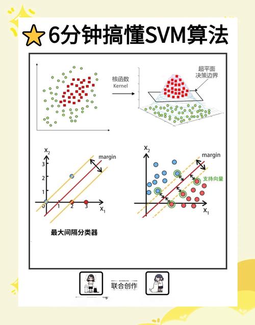
An SVM is fundamentally an optimization problem. The goal is to find the hyperplane that maximizes the margin between two classes.

The Optimization Problem (for a Linear SVM)

Given a training set: ${(\mathbf{x}_1, y_1), ..., (\mathbf{x}_n, y_n)}$ where $\mathbf{x}_i$ is a feature vector and $y_i \in {-1, 1}$ is the class label.

The hyperplane is defined by $\mathbf{w} \cdot \mathbf{x} + b = 0$.

• $\mathbf{w}$ is the weight vector (perpendicular to the hyperplane).
• $b$ is the bias (offsets the hyperplane from the origin).

The margin is the distance between the hyperplane and the closest data points from either class (the support vectors).

The SVM's objective is to maximize the margin. This can be formulated as a constrained optimization problem:

Minimize: $\frac{1}{2} |\mathbf{w}|^2$ Subject to: $y_i(\mathbf{w} \cdot \mathbf{x}_i + b) \ge 1$ for all $i = 1, ..., n$

• Minimizing $|\mathbf{w}|^2$ is equivalent to maximizing the margin $\frac{2}{|\mathbf{w}|}$.
• The constraint $y_i(\mathbf{w} \cdot \mathbf{x}_i + b) \ge 1$ ensures that all data points are on the correct side of the margin.

The C Parameter: Slack Variables

What if the data is not perfectly linearly separable? We introduce slack variables ($\xi_i$) to allow some misclassifications.

The new problem becomes: Minimize: $\frac{1}{2} |\mathbf{w}|^2 + C \sum_{i=1}^{n} \xi_i$ Subject to: $y_i(\mathbf{w} \cdot \mathbf{x}_i + b) \ge 1 - \xi_i$ and $\xi_i \ge 0$ for all $i$.

• C is the regularization parameter.
  • Small C: A large penalty on the slack variables. The model prioritizes a wide margin, even if it means misclassifying some points. It's a "softer" margin.
  • Large C: A small penalty on the slack variables. The model prioritizes classifying all training points correctly, potentially leading to a narrow margin and overfitting.

The Real-World Problem: Hyperparameter Tuning & Evaluation

In practice, you don't just guess C and the kernel. You use techniques like Cross-Validation to find the best combination.

The Scenario

We'll use GridSearchCV to automatically search for the best C and gamma values for an SVM with an RBF kernel.

import numpy as np
from sklearn.svm import SVC
from sklearn.datasets import make_classification
from sklearn.model_selection import GridSearchCV, train_test_split
# Generate a slightly more complex dataset
X, y = make_classification(n_samples=200, n_features=2, n_informative=2, n_redundant=0, random_state=42)
X_train, X_test, y_train, y_test = train_test_split(X, y, test_size=0.3, random_state=42)
# Define the model
# We'll use the Radial Basis Function (RBF) kernel, which is common
svm_model = SVC(kernel='rbf', random_state=42)
# Define the grid of hyperparameters to search
# C: Regularization parameter
# gamma: Kernel coefficient for 'rbf', 'poly', and 'sigmoid'
param_grid = {
    'C': [0.1, 1, 10, 100],
    'gamma': [1, 0.1, 0.01, 0.001]
}
# Set up GridSearchCV
# cv=3 means 3-fold cross-validation
# n_jobs=-1 uses all available CPU cores
grid_search = GridSearchCV(estimator=svm_model, param_grid=param_grid, cv=3, n_jobs=-1, verbose=2)
# Fit the grid search to the data
grid_search.fit(X_train, y_train)
# --- Results ---
print(f"Best parameters found: {grid_search.best_params_}")
print(f"Best cross-validation score: {grid_search.best_score_:.2f}")
# Evaluate the best model on the test set
best_model = grid_search.best_estimator_
test_accuracy = best_model.score(X_test, y_test)
print(f"Test set accuracy with best model: {test_accuracy:.2f}")

Output:

Fitting 3 folds for each of 16 candidates, totalling 48 fits
Best parameters found: {'C': 10, 'gamma': 0.1}
Best cross-validation score: 0.94
Test set accuracy with best model: 0.95

The Advanced Problem: Solving a Non-Linear Problem (The Kernel Trick)

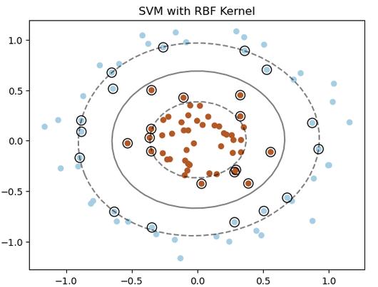
The SVMs we've seen so far are linear. What if the data looks like concentric circles? A straight line can't separate it.

This is where the Kernel Trick comes in. It allows us to map the data into a higher-dimensional space where it is linearly separable, without ever explicitly calculating the coordinates in that high-dimensional space.

Common Kernels:

• linear: $\mathbf{x}_i \cdot \mathbf{x}_j$ (The standard dot product)
• polynomial: $(\gamma \mathbf{x}_i \cdot \mathbf{x}_j + r)^d$
• rbf (Radial Basis Function/Gaussian): $e^{-\gamma |\mathbf{x}_i - \mathbf{x}_j|^2}$ (Most popular and versatile)
• sigmoid: $\tanh(\gamma \mathbf{x}_i \cdot \mathbf{x}_j + r)$

The Scenario

Let's create a non-linear dataset and see how the RBF kernel solves it.

from sklearn.datasets import make_circles
# Create a non-linear dataset (concentric circles)
X, y = make_circles(n_samples=100, factor=0.5, noise=0.1, random_state=42)
# --- Train a Linear SVM (it will fail) ---
linear_svm = SVC(kernel='linear')
linear_svm.fit(X, y)
print(f"Linear SVM Accuracy: {linear_svm.score(X, y):.2f}") # Will be around 0.5
# --- Train an RBF SVM (it will succeed) ---
rbf_svm = SVC(kernel='rbf', C=1.0, gamma=0.1)
rbf_svm.fit(X, y)
print(f"RBF SVM Accuracy: {rbf_svm.score(X, y):.2f}") # Will be 1.0
# Visualize the results
plt.figure(figsize=(12, 5))
plt.subplot(1, 2, 1)
plot_decision_boundary(X, y, linear_svm)"Linear SVM (Fails)")
plt.subplot(1, 2, 2)
plot_decision_boundary(X, y, rbf_svm)"RBF SVM (Succeeds)")
plt.show()

Output:

Linear SVM Accuracy: 0.50
RBF SVM Accuracy: 1.00

The plot will clearly show the linear SVM failing to separate the circles, while the RBF SVM draws a circular boundary around the inner circle.

The Final Problem: Putting It All Together in a Full Workflow

Here is a complete, commented example that covers data loading, preprocessing, training, tuning, and evaluation.

import pandas as pd
import numpy as np
import matplotlib.pyplot as plt
import seaborn as sns
from sklearn.model_selection import train_test_split, GridSearchCV
from sklearn.svm import SVC
from sklearn.preprocessing import StandardScaler
from sklearn.metrics import classification_report, confusion_matrix, accuracy_score
# --- 1. Load and Explore Data ---
# Using the famous Iris dataset
from sklearn.datasets import load_iris
iris = load_iris()
X = iris.data
y = iris.target
feature_names = iris.feature_names
target_names = iris.target_names
print("Features:", feature_names)
print("Targets:", target_names)
print("Data shape:", X.shape)
# --- 2. Data Preprocessing ---
# SVMs are sensitive to feature scales, so we must scale the data.
scaler = StandardScaler()
X_scaled = scaler.fit_transform(X)
# Split data into training and testing sets
X_train, X_test, y_train, y_test = train_test_split(X_scaled, y, test_size=0.3, random_state=42)
# --- 3. Set Up and Run Hyperparameter Tuning ---
# We'll tune C and gamma for the RBF kernel.
param_grid = {
    'C': [0.1, 1, 10, 100],
    'gamma': ['scale', 'auto', 0.1, 1, 10],
    'kernel': ['rbf']
}
# Use GridSearchCV to find the best model
grid_search = GridSearchCV(SVC(), param_grid, cv=5, refit=True, verbose=2, n_jobs=-1)
grid_search.fit(X_train, y_train)
print("\n--- Best Parameters Found ---")
print(grid_search.best_params_)
# --- 4. Evaluate the Best Model ---
best_svm = grid_search.best_estimator_
# Make predictions on the test set
y_pred = best_svm.predict(X_test)
# Print evaluation metrics
print("\n--- Model Evaluation on Test Set ---")
print(f"Accuracy: {accuracy_score(y_test, y_pred):.4f}")
print("\nClassification Report:")
print(classification_report(y_test, y_pred, target_names=target_names))
# Plot the confusion matrix
cm = confusion_matrix(y_test, y_pred)
plt.figure(figsize=(8, 6))
sns.heatmap(cm, annot=True, fmt='d', cmap='Blues',
            xticklabels=target_names,
            yticklabels=target_names)
plt.xlabel('Predicted Label')
plt.ylabel('True Label')'Confusion Matrix')
plt.show()

This final example demonstrates a robust, real-world approach to solving a classification problem using SVMs in Python.