Of course. Using Python 2.7 with TFLearn is a combination that was popular in the mid-to-late 2010s. It's important to understand that this is an older, deprecated stack. Modern development strongly recommends using Python 3 and a more current deep learning framework like TensorFlow 2.x or PyTorch.

However, if you have a specific reason to use this older combination (e.g., maintaining a legacy project), here is a comprehensive guide covering the setup, concepts, and a complete example.
Important Context: Why This Stack is Deprecated
- Python 2.7 End-of-Life: Python 2.7 officially reached its end-of-life in January 2025. It no longer receives security updates, bug fixes, or improvements. Using it is a security risk and not recommended for new projects.
- TFLearn is Inactive: The TFLearn library has not seen significant updates since around 2025. It was built on top of TensorFlow 1.x. It does not work with modern TensorFlow 2.x.
- Modern Alternatives: The deep learning ecosystem has moved on. TensorFlow 2.x (with its
tf.kerasAPI) and PyTorch are the current standards. They are more powerful, easier to use, better supported, and actively developed.
Recommendation: If possible, plan to migrate your project to Python 3 and TensorFlow 2.x. This guide is for maintaining legacy systems only.
Installation for Python 2.7
The key is to install the correct versions of each library that are compatible with Python 2.7.
Step 1: Create a Virtual Environment (Highly Recommended)

This isolates your project's dependencies from your system's Python installation.
# Make sure you have Python 2.7 installed and in your PATH
python --version  # Should show Python 2.7.x
# Create a virtual environment named 'tflearn_py27'
virtualenv tflearn_py27
# Activate the virtual environment
# On Windows:
tflearn_py27\Scripts\activate
# On macOS/Linux:
source tflearn_py27/bin/activate
Step 2: Install Dependencies
Now, inside your activated virtual environment, install the specific versions.
# Install TFLearn (this will automatically install compatible TensorFlow 1.x and NumPy)
pip install tflearn
# At the time of writing, this typically installs:
# - TFLearn
# - TensorFlow 1.x (e.g., 1.15)
# - NumPy 1.x (e.g., 1.18)
# - six
You can verify the installation:

# Check Python version
python --version
# Check installed packages
pip list
# You should see tflearn, tensorflow, numpy, etc.
Core Concepts of TFLearn
TFLearn provides a high-level, layer-based API for building neural networks on top of TensorFlow. It simplifies many of the lower-level details.
Key Components:
input_data: A placeholder for your training data. It defines the shape of your input tensors.DNN(Deep Neural Network): A helper function to easily build a standard feed-forward network with multiple hidden layers.fully_connected: A standard, fully connected neural network layer.dropout: A regularization technique to prevent overfitting.regression: An output layer for regression tasks (predicting a continuous value).classification: An output layer for classification tasks.fit: The method to train the model on your data.predict: The method to use the trained model for making predictions.
Complete Example: Iris Flower Classification
This classic example demonstrates how to build, train, and evaluate a simple neural network to classify iris flowers into one of three species.
The Code (iris_classifier.py)
# -*- coding: utf-8 -*-
import tflearn
from tflearn.data_utils import load_csv
import numpy as np
# --- 1. Load and Preprocess Data ---
# Load the dataset. The dataset is a CSV file.
# The first 4 columns are features (sepal length, sepal width, petal length, petal width).
# The 5th column is the label (species of iris).
data_file = 'iris.csv'
# We specify that the last column is the target/label
data, labels = load_csv(data_file, target_column=-1, categorical_labels=True, n_classes=3)
# --- 2. Build the Neural Network ---
# Reset the graph to ensure a clean model
tflearn.init_graph()
# Define the input layer. It expects 4 features.
net = tflearn.input_data(shape=[None, 4])
# Build the network:
# - Two fully-connected hidden layers with 32 neurons each.
# - 'activation='relu'' is the Rectified Linear Unit activation function.
# - 'dropout=0.5' applies dropout for regularization to prevent overfitting.
net = tflearn.fully_connected(net, 32, activation='relu')
net = tflearn.dropout(net, 0.8)
net = tflearn.fully_connected(net, 32, activation='relu')
net = tflearn.dropout(net, 0.8)
# Define the output layer.
# - 'n_classes=3' because there are 3 species of iris.
# - 'activation='softmax'' is used for multi-class classification.
net = tflearn.fully_connected(net, 3, activation='softmax')
# Define the regression layer. It connects the network to the loss function.
# 'optimizer='adam'' is an efficient gradient descent algorithm.
# 'loss='categorical_crossentropy'' is the standard loss function for multi-class classification.
net = tflearn.regression(net, optimizer='adam', loss='categorical_crossentropy')
# --- 3. Train the Model ---
# Build the DNN model
model = tflearn.DNN(net)
# Train the model
# 'n_epoch=50' means we'll go through the entire dataset 50 times.
# 'show_metric=True' will display the accuracy and loss during training.
print("Training model...")
model.fit(data, labels, n_epoch=50, batch_size=16, show_metric=True)
# --- 4. Evaluate and Use the Model ---
print("Training complete.")
# Let's make a prediction on a new, unseen flower
# Example: Sepal Length=5.1, Sepal Width=3.5, Petal Length=1.4, Petal Width=0.2 (this is an Iris-setosa)
new_flower = np.array([[5.1, 3.5, 1.4, 0.2]])
# Predict the class
prediction = model.predict(new_flower)
# The output will be an array of probabilities for each class
print("\nPrediction for new flower:", prediction)
# Get the class with the highest probability
predicted_class = np.argmax(prediction, axis=1)
print("Predicted class index:", predicted_class)
# You can map the index back to the species name if you have the mapping
# For example: 0 -> 'setosa', 1 -> 'versicolor', 2 -> 'virginica'
species_names = ['setosa', 'versicolor', 'virginica']
print("Predicted species:", species_names[predicted_class[0]])
How to Run the Example
- Save the Code: Save the code above as
iris_classifier.py. - Get the Data: Download the
iris.csvfile. You can find it easily online (e.g., from the UCI Machine Learning Repository). Make sure it's in the same directory as your Python script.- UCI Iris Dataset CSV
- You may need to add a header row to the CSV:
sepal_length,sepal_width,petal_length,petal_width,species.
- Execute:
# Make sure your virtual environment is activated
python iris_classifier.py
You will see the training progress, with the accuracy increasing and the loss decreasing over the 50 epochs. Finally, it will predict the species for the new flower example.