Of course! Python is the undisputed king of data mining. Its rich ecosystem of open-source libraries makes it incredibly powerful, flexible, and accessible for everyone from beginners to seasoned data scientists.
This guide will walk you through the entire data mining process using Python, from setting up your environment to building and evaluating predictive models.
What is Data Mining?
In simple terms, data mining is the process of discovering patterns, correlations, and anomalies within large datasets to extract useful information. It's not about just looking at data; it's about using algorithms to automatically discover hidden knowledge.
The process typically follows these steps, which we'll cover in detail:
- Data Collection & Loading: Getting your data into Python.
- Data Cleaning & Preprocessing: Handling missing values, correcting errors, and formatting data.
- Exploratory Data Analysis (EDA): Understanding the data through visualization and statistics.
- Feature Engineering: Creating new, more meaningful features from existing data.
- Model Building: Choosing and training a machine learning model.
- Model Evaluation: Assessing how well your model performs.
- Deployment (Conceptual): Using the model to make predictions on new data.
The Essential Python Data Mining Toolkit
You don't need to reinvent the wheel. Python has a library for almost every step of the process.
| Task | Primary Libraries | What they do |
|---|---|---|
| Data Manipulation | Pandas, NumPy | The backbone. Pandas provides DataFrames for handling tabular data. NumPy provides powerful numerical operations. |
| Data Visualization | Matplotlib, Seaborn | Matplotlib is the foundational plotting library. Seaborn builds on it to create beautiful, statistical plots with less code. |
| Machine Learning | Scikit-learn | The go-to library for classical machine learning. It provides simple and efficient tools for data mining and analysis. |
| Deep Learning (Advanced) | TensorFlow, PyTorch | For complex tasks like image recognition and natural language processing. |
| Data Access | SQLAlchemy, Pymongo | For connecting to SQL databases and NoSQL databases like MongoDB. |
A Step-by-Step Data Mining Example in Python
Let's walk through a classic data mining task: predicting customer churn. We'll use a public dataset from Telco, where we want to predict which customers are likely to leave the service.
Step 0: Setup
First, make sure you have the necessary libraries installed. Open your terminal or command prompt and run:
pip install pandas numpy matplotlib seaborn scikit-learn
Step 1: Data Collection & Loading
We'll load the dataset directly from a URL into a Pandas DataFrame.
import pandas as pd
import numpy as np
# Load the dataset
# Using a sample dataset from a public repository
url = "https://raw.githubusercontent.com/IBM/telco-customer-churn-on-icp4d/master/data/Telco-Customer-Churn.csv"
df = pd.read_csv(url)
# Display the first 5 rows of the dataframe
print(df.head())
# Get a concise summary of the dataframe
print(df.info())
Step 2: Data Cleaning & Preprocessing
Real-world data is messy. This is often the most time-consuming but crucial step.
# --- 2a. Handle Missing Values ---
# The 'TotalCharges' column has empty strings that need to be converted to NaN
df['TotalCharges'] = pd.to_numeric(df['TotalCharges'], errors='coerce')
# Check for missing values
print(df.isnull().sum())
# We have 11 missing values in 'TotalCharges'. Let's fill them with the median.
df['TotalCharges'].fillna(df['TotalCharges'].median(), inplace=True)
# --- 2b. Handle Categorical Data ---
# Machine learning models need numbers, not text. We'll convert categorical columns.
# The 'Churn' column is our target variable. Let's map it to 1 and 0.
df['Churn'] = df['Churn'].map({'Yes': 1, 'No': 0})
# For other categorical features, we can use One-Hot Encoding
# This creates new binary (0/1) columns for each category.
# We'll drop the first column to avoid multicollinearity.
df = pd.get_dummies(df, columns=['gender', 'Partner', 'Dependents', 'PhoneService',
                                 'MultipleLines', 'InternetService', 'OnlineSecurity',
                                 'OnlineBackup', 'DeviceProtection', 'TechSupport',
                                 'StreamingTV', 'StreamingMovies', 'Contract',
                                 'PaperlessBilling', 'PaymentMethod'], drop_first=True)
# --- 2c. Drop Unnecessary Columns ---
# The 'customerID' is just an identifier and not useful for prediction.
df.drop('customerID', axis=1, inplace=True)
print("\nData after preprocessing:")
print(df.head())
Step 3: Exploratory Data Analysis (EDA)
Now, let's explore the data to understand it better.
import matplotlib.pyplot as plt
import seaborn as sns
# --- 3a. Visualize the Target Variable ---
plt.figure(figsize=(6, 4))
sns.countplot(x='Churn', data=df)'Churn Distribution')
plt.show()
# This shows us that we have an imbalanced dataset (more non-churners than churners).
# --- 3b. Explore Relationships ---
# Let's see how 'MonthlyCharges' relates to churn.
plt.figure(figsize=(10, 6))
sns.histplot(data=df, x='MonthlyCharges', hue='Churn', kde=True, element='step')'Monthly Charges vs. Churn')
plt.show()
# This plot might suggest that customers with higher monthly charges are more likely to churn.
# --- 3c. Correlation Heatmap ---
plt.figure(figsize=(15, 10))
correlation_matrix = df.corr()
sns.heatmap(correlation_matrix, annot=False, cmap='coolwarm')'Correlation Matrix of Features')
plt.show()
# This helps identify which features are most correlated with each other and with our target 'Churn'.
Step 4: Feature Engineering
Sometimes, creating new features can improve model performance. For this example, let's create a simple feature: the ratio of TotalCharges to tenure.
# Avoid division by zero for new customers
df['ChargesPerTenure'] = df['TotalCharges'] / (df['tenure'] + 1)
print("\nData after feature engineering:")
print(df[['tenure', 'TotalCharges', 'ChargesPerTenure']].head())
Step 5: Model Building
We'll split our data into training and testing sets and then train a model.
from sklearn.model_selection import train_test_split
from sklearn.ensemble import RandomForestClassifier
# --- 5a. Define Features (X) and Target (y) ---
X = df.drop('Churn', axis=1) # All columns except 'Churn'
y = df['Churn'] # The 'Churn' column
# --- 5b. Split the data into training and testing sets ---
# 80% for training, 20% for testing
X_train, X_test, y_train, y_test = train_test_split(X, y, test_size=0.2, random_state=42, stratify=y)
# --- 5c. Initialize and Train the Model ---
# We'll use a Random Forest, which is a powerful and popular ensemble method.
model = RandomForestClassifier(n_estimators=100, random_state=42)
print("\nTraining the model...")
model.fit(X_train, y_train)
print("Model training complete.")
Step 6: Model Evaluation
How good is our model? We'll use several metrics to evaluate its performance on the unseen test data.
from sklearn.metrics import accuracy_score, confusion_matrix, classification_report
# --- 6a. Make Predictions on the Test Set ---
y_pred = model.predict(X_test)
# --- 6b. Evaluate the Model ---
accuracy = accuracy_score(y_test, y_pred)
print(f"\nModel Accuracy: {accuracy:.4f}")
# --- 6c. Confusion Matrix ---
# A confusion matrix shows us where the model got confused.
cm = confusion_matrix(y_test, y_pred)
plt.figure(figsize=(8, 6))
sns.heatmap(cm, annot=True, fmt='d', cmap='Blues', xticklabels=['No Churn', 'Churn'], yticklabels=['No Churn', 'Churn'])
plt.xlabel('Predicted')
plt.ylabel('Actual')'Confusion Matrix')
plt.show()
# --- 6d. Classification Report ---
# This gives precision, recall, and F1-score, which are crucial for imbalanced datasets.
print("\nClassification Report:")
print(classification_report(y_test, y_pred, target_names=['No Churn', 'Churn']))
Interpreting the Classification Report:
- Precision: Of all the customers the model predicted would churn, how many actually did?
- Recall: Of all the customers that actually churned, how many did the model correctly identify?
- F1-Score: A weighted average of precision and recall.
Step 7: Feature Importance
A great benefit of models like Random Forest is that they can tell you which features were most important for making predictions.
# Get feature importances from the trained model
importances = model.feature_importances_
feature_names = X.columns
# Create a DataFrame for visualization
feature_importance_df = pd.DataFrame({'feature': feature_names, 'importance': importances})
feature_importance_df = feature_importance_df.sort_values(by='importance', ascending=False)
# Plot the top 10 most important features
plt.figure(figsize=(12, 8))
sns.barplot(x='importance', y='feature', data=feature_importance_df.head(10))'Top 10 Most Important Features for Predicting Churn')
plt.show()
This plot can provide actionable business insights, for example: "It seems that tenure and Contract_Month-to-month are the biggest drivers of customer churn."
Where to Go from Here
This example covers the fundamentals. To become a true data mining expert, you should explore:
- More Algorithms: Try
Logistic Regression,Support Vector Machines (SVM),Gradient Boosting (XGBoost, LightGBM). - Advanced Preprocessing: Learn about
Feature Scaling(StandardScaler,MinMaxScaler),Dimensionality Reduction(PCA), and handling more complex categorical data. - Hyperparameter Tuning: Use
GridSearchCVorRandomizedSearchCVto find the optimal settings for your model. - Deep Learning: For unstructured data like images and text, explore TensorFlow and PyTorch.
- Big Data Tools: For datasets that don't fit in memory, learn about
DaskorPySpark.


