Of course! Deconvolution is a powerful signal processing technique used to reverse the effect of convolution. In simpler terms, if you have a "blurred" or "noisy" signal and you know the cause of the blur (the "kernel" or "point spread function"), deconvolution helps you recover the original, sharp signal.

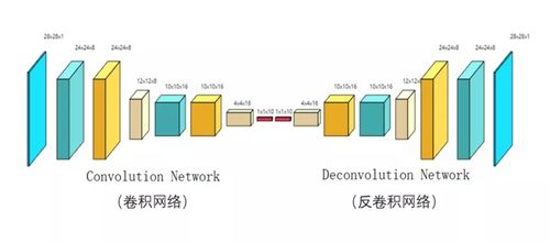
This is a common problem in many fields:

• Image Processing: Sharpening a blurry photo, removing motion blur, or correcting for a blurry lens.
• Astronomy: Restoring sharp images of celestial objects that have been blurred by atmospheric turbulence (seeing).
• Seismology: Determining the original source of an earthquake wave after it has traveled through and been distorted by the Earth's layers.
• Medical Imaging: Improving the quality of MRI or CT scans.

Let's break down how to perform deconvolution in Python, starting with the core concepts and moving to practical code examples.

The Core Concept: Convolution and Deconvolution

Convolution is the process of combining two signals (a signal and a kernel) to produce a third signal. It's often described as a "sliding window" operation where the kernel is slid over the signal, and at each point, a weighted sum is calculated.

Mathematically: (signal * kernel)(t) = ∫ signal(τ) kernel(t - τ) dτ

In the real world, we often observe a convolved signal: observed_signal = true_signal * kernel + noise

Deconvolution is the inverse operation. Given the observed_signal and the kernel, our goal is to estimate the true_signal.

estimated_true_signal = deconv(observed_signal, kernel)

Key Methods for Deconvolution

There are several ways to perform deconvolution, each with its own trade-offs between speed, accuracy, and sensitivity to noise.

1. Direct Inverse in the Frequency Domain (Wiener Deconvolution - a simplified case)

   • How it works: This is the most intuitive method. It leverages the Convolution Theorem, which states that convolution in the time/space domain is equivalent to element-wise multiplication in the frequency domain.
     • Take the FFT of the observed signal.
     • Take the FFT of the kernel.
     • In the frequency domain, "divide" the signal's spectrum by the kernel's spectrum.
     • Take the Inverse FFT to get the deconvolved signal.
   • The Problem: If the kernel's spectrum has values close to zero, this division becomes unstable and amplifies noise immensely. This is called "ill-posedness."

2. Wiener Deconvolution

   • How it works: This is a massive improvement over the direct inverse. It incorporates knowledge about the signal-to-noise ratio (SNR) to prevent noise amplification. Instead of just dividing by H(f) (the kernel's FFT), it divides by a more stable term.
   • Pros: Very effective when you have an estimate of the noise level. It's a classic and widely used method.
   • Cons: Requires you to know or estimate the noise power.

3. Richardson-Lucy Deconvolution

   • How it works: This is an iterative algorithm commonly used in astronomy and fluorescence microscopy. It's based on Bayesian statistics and is particularly good for signals that are positive (like light intensity or photon counts).
   • Pros: Excellent at preserving signal structure and is less prone to amplifying negative artifacts than Wiener deconvolution. It works well even with low signal-to-noise ratios.
   • Cons: Computationally intensive due to iteration. Can sometimes introduce "ringing" artifacts if not stopped at the right time.

Practical Python Implementation

We'll use scipy.signal and numpy for our examples.

Setup and Sample Data

First, let's create a sample 1D signal, blur it with a known kernel, and add some noise. This simulates a real-world observation.

import numpy as np
import matplotlib.pyplot as plt
from scipy.signal import convolve, wiener, richardson_lucy
from scipy.fft import fft, ifft, fftfreq
# --- 1. Create a Sample Signal ---
# A clean signal with some features
original_signal = np.zeros(200)
original_signal[50:70] = 10  # A sharp peak
original_signal[80:100] = 5  # A plateau
original_signal[120:140] = 8 # Another peak
# --- 2. Create a Blurring Kernel ---
# A simple Gaussian kernel (simulates a point spread function)
kernel_size = 11
kernel = np.exp(-np.linspace(-2, 2, kernel_size)**2)
kernel /= kernel.sum() # Normalize the kernel
# --- 3. Convolve the Signal with the Kernel ---
# This simulates the "observed" or "blurred" signal
blurred_signal = convolve(original_signal, kernel, mode='same')
# --- 4. Add Noise ---
# Real-world data always has noise
noise = np.random.normal(0, 0.5, blurred_signal.shape)
observed_signal = blurred_signal + noise
# --- Plotting the Setup ---
plt.figure(figsize=(12, 6))
plt.plot(original_signal, label='Original Signal', linewidth=2)
plt.plot(blurred_signal, label='Blurred Signal (No Noise)', linestyle='--')
plt.plot(observed_signal, label='Observed Signal (with Noise)', alpha=0.7)'Signal Before and After Blurring')
plt.xlabel('Sample')
plt.ylabel('Amplitude')
plt.legend()
plt.grid(True)
plt.show()

Now, let's try to recover the original signal from observed_signal and our kernel.

Method 1: Wiener Deconvolution

The scipy.signal.wiener function is very easy to use. The key parameter is noise, which is an estimate of the noise-to-signal power ratio. If you don't know it, you can experiment with small values (e.g., 0.01 to 0.1).

# Perform Wiener deconvolution
# The 'noise' parameter is crucial. It's the noise power / signal power ratio.
# You may need to tune this for your specific data.
wiener_deconvolved = wiener(observed_signal, noise=0.05, mysize=kernel_size)
# --- Plotting the Result ---
plt.figure(figsize=(12, 6))
plt.plot(original_signal, label='Original Signal', linewidth=2)
plt.plot(observed_signal, label='Observed Signal', alpha=0.7)
plt.plot(wiener_deconvolved, label='Wiener Deconvolution', linestyle=':')'Wiener Deconvolution Result')
plt.xlabel('Sample')
plt.ylabel('Amplitude')
plt.legend()
plt.grid(True)
plt.show()

Result Analysis: The Wiener filter does a decent job of recovering the general shape of the signal. It smooths out some noise but can also slightly blur the sharp edges. The result is highly dependent on the noise parameter.

Method 2: Richardson-Lucy Deconvolution

The scipy.signal.richardson_lucy function is also straightforward. It requires the number of iterations (num_iter). More iterations can recover more detail but also risk amplifying noise and artifacts.

# Perform Richardson-Lucy deconvolution
# The number of iterations is a critical parameter to tune.
rl_deconvolved = richardson_lucy(observed_signal, kernel, num_iter=30, clip=False)
# --- Plotting the Result ---
plt.figure(figsize=(12, 6))
plt.plot(original_signal, label='Original Signal', linewidth=2)
plt.plot(observed_signal, label='Observed Signal', alpha=0.7)
plt.plot(rl_deconvolved, label='Richardson-Lucy Deconvolution', linestyle='-.')'Richardson-Lucy Deconvolution Result')
plt.xlabel('Sample')
plt.ylabel('Amplitude')
plt.legend()
plt.grid(True)
plt.show()

Result Analysis: The Richardson-Lucy algorithm often produces sharper results than Wiener deconvolution. It's better at preserving the peak structures. However, you might notice some small "ringing" artifacts near sharp edges, especially if you run too many iterations. The clip=False argument allows the result to have negative values, which can be useful for some signals.

Method 3: Manual Frequency Domain Deconvolution (for educational purposes)

This demonstrates the "direct inverse" method and clearly shows its weakness with noise.

def manual_deconvolution(signal, kernel):
    """Performs deconvolution in the frequency domain."""
    # Pad the kernel to the same length as the signal
    padded_kernel = np.zeros_like(signal)
    padded_kernel[:len(kernel)] = kernel
    # Compute FFTs
    signal_fft = fft(signal)
    kernel_fft = fft(padded_kernel)
    # Avoid division by zero
    # A small epsilon is added to prevent division by zero
    epsilon = 1e-10 
    deconv_fft = signal_fft / (kernel_fft + epsilon)
    # Inverse FFT to get the result in