Of course! Creating pivot tables in Python is a common and powerful data analysis task. While you might be familiar with pivot tables in Excel, Python offers more flexibility and programmatic control.

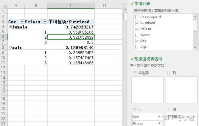
The primary tool for this in Python is the Pandas library. I'll guide you through it, starting with the basics and moving to more advanced examples.

The Core Idea

A pivot table is a data summarization tool. It allows you to:

1. Group your data by one or more categories.
2. Aggregate (e.g., sum, mean, count) a numerical column based on those groups.
3. Re-orient the data to present it in a clear, tabular format.

The Setup: Importing Libraries and Creating Data

First, you need to have Pandas installed. If you don't, run:

pip install pandas

Now, let's import Pandas and create a sample DataFrame to work with. This DataFrame represents sales data.

import pandas as pd
import numpy as np
# Create a sample DataFrame
data = {
    'Date': pd.to_datetime(['2025-01-15', '2025-01-15', '2025-02-20', '2025-02-20', '2025-03-10', '2025-03-10', '2025-03-10']),
    'Region': ['East', 'West', 'East', 'West', 'East', 'West', 'Central'],
    'Salesperson': ['Alice', 'Bob', 'Alice', 'Bob', 'Charlie', 'Bob', 'David'],
    'Product': ['A', 'B', 'A', 'B', 'A', 'B', 'C'],
    'Units_Sold': [100, 150, 120, 180, 90, 200, 75],
    'Revenue': [10000, 15000, 12000, 18000, 9000, 20000, 11250] # Revenue = Units_Sold * 100 (simplified)
}
df = pd.DataFrame(data)
print("Original DataFrame:")
print(df)

Original DataFrame:

        Date Region Salesperson Product  Units_Sold  Revenue
0 2025-01-15   East       Alice       A         100    10000
1 2025-01-15    West         Bob       B         150    15000
2 2025-02-20   East       Alice       A         120    12000
3 2025-02-20    West         Bob       B         180    18000
4 2025-03-10   East     Charlie       A          90     9000
5 2025-03-10    West         Bob       B         200    20000
6 2025-03-10  Central       David       C          75    11250

The Basic Pivot Table: pd.pivot_table()

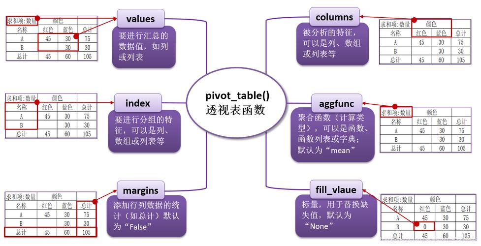
The function pd.pivot_table() is the workhorse. Its most important arguments are:

• data: The DataFrame you want to pivot.
• values: The numerical column you want to aggregate.
• index: The column(s) you want to become the new rows of your pivot table.
• columns: The column(s) you want to become the new columns of your pivot table.
• aggfunc: The function to use for aggregation (e.g., 'sum', 'mean', 'count', 'max'). Default is 'mean'.
• fill_value: A value to replace missing data (NaNs) with.

Example 1: Total Revenue by Region and Product

Let's find the total Revenue for each Region and Product.

# Pivot to see total revenue by region and product
pivot_revenue = pd.pivot_table(
    data=df,
    values='Revenue',
    index='Region',
    columns='Product',
    aggfunc='sum',
    fill_value=0 # Replace NaN with 0
)
print("\nPivot Table: Total Revenue by Region and Product")
print(pivot_revenue)

Result:

Pivot Table: Total Revenue by Region and Product
Product       A      B       C
Region
Central     0      0   11250
East     31000      0       0
West        0  53000       0

• index='Region': Central, East, and West become the row labels.
• columns='Product': A, B, and C become the column headers.
• values='Revenue': We are summarizing the Revenue column.
• aggfunc='sum': We are summing the revenue for each combination.

Common Aggregation Functions

You can easily switch the aggregation method.

Example 2: Average Units Sold by Salesperson

Let's find the average Units_Sold for each Salesperson.

# Pivot to see average units sold by salesperson
pivot_avg_units = pd.pivot_table(
    data=df,
    values='Units_Sold',
    index='Salesperson',
    aggfunc='mean'
)
print("\nPivot Table: Average Units Sold by Salesperson")
print(pivot_avg_units.round(2)) # Round for cleaner output

Result:

Pivot Table: Average Units Sold by Salesperson
               Units_Sold
Salesperson              
Alice           110.00
Bob            176.67
Charlie         90.00
David           75.00

Example 3: Count of Sales by Region

To count the number of sales, you can use aggfunc='count' or len. A common trick is to use a column that never has missing values, like the Date.

# Pivot to count the number of sales by region
pivot_sales_count = pd.pivot_table(
    data=df,
    values='Date', # Using Date to count transactions
    index='Region',
    aggfunc='count'
)
print("\nPivot Table: Count of Sales by Region")
print(pivot_sales_count)

Result:

Pivot Table: Count of Sales by Region
        Date
Region
Central     1
East        2
West        3

Using Multiple Indexes and Columns (Hierarchical Indexing)

Pandas allows you to use multiple columns for your index and columns parameters, creating a more detailed and hierarchical pivot table.

Example 4: Monthly Revenue by Region and Product

Let's break down the revenue by Date (month), Region, and Product.

# Add a 'Month' column for easier grouping
df['Month'] = df['Date'].dt.to_period('M')
# Pivot with multiple index and columns
pivot_multi = pd.pivot_table(
    data=df,
    values='Revenue',
    index=['Month', 'Region'], # Multi-level index
    columns='Product',          # Single level column
    aggfunc='sum',
    fill_value=0
)
print("\nPivot Table: Monthly Revenue by Region and Product (Multi-level Index)")
print(pivot_multi)

Result:

Pivot Table: Monthly Revenue by Region and Product (Multi-level Index)
Product            A       B       C
Month   Region
2025-01 Central     0       0       0
        East    10000       0       0
        West        0  15000       0
2025-02 Central     0       0       0
        East    12000       0       0
        West        0  18000       0
2025-03 Central     0       0  11250
        East     9000       0       0
        West        0  20000       0

Notice the Month and Region are now a multi-level index. You can access sub-levels like this:

print(pivot_multi.loc['2025-01'])

Multiple Aggregation Functions

What if you want to see both the sum and the average in the same table? You can pass a list of functions to aggfunc.

Example 5: Sum and Average of Units Sold by Region

# Pivot with multiple aggregation functions
pivot_multi_agg = pd.pivot_table(
    data=df,
    values='Units_Sold',
    index='Region',
    aggfunc=['sum', 'mean', 'max'] # List of aggregation functions
)
print("\nPivot Table: Multiple Aggregations for Units Sold by Region")
print(pivot_multi_agg.round(2))

Result:

Pivot Table: Multiple Aggregations for Units Sold by Region
       sum       mean    max
Units_Sold Units_Sold Units_Sold
Region
Central           75      75.00     75
East            310     103.33    120
West            530     176.67    200

The column names become multi-level as well.

The Alternative: .groupby().unstack()

For more complex or programmatic operations, you can achieve the same result (and more) using a two-step process: groupby() followed by unstack().

• groupby(): Groups the data.
• unstack(): Pivots the innermost level of the index into columns.

This is often more intuitive for those coming from a SQL background.

Example 6: Recreating Example 1 with groupby().unstack()

# Group by Region and Product, then sum the Revenue
grouped = df.groupby(['Region', 'Product'])['Revenue'].sum().reset_index()
# Unstack the 'Product' level to make it columns
pivot_from_groupby = grouped.set_index(['Region', 'Product']).unstack()
# The result has a multi-level column, so we can clean it up
pivot_from_groupby.columns = pivot_from_groupby.columns.droplevel(0)
pivot_from_groupby = pivot_from_groupby.fill_value(0)
print("\nPivot Table created with groupby().unstack()")
print(pivot_from_groupby)

This produces the exact same output as Example 1. The choice between pivot_table() and groupby().unstack() is often a matter of style and complexity. pivot_table() is more direct for standard pivot tasks, while groupby().unstack() offers more flexibility for custom aggregation chains.

Summary: When to Use Which

For most day-to-day data analysis, pd.pivot_table() is your best friend. It's the direct equivalent of Excel's pivot table functionality and is incredibly efficient.