Of course! Let's break down how to find and use a threshold for an AUC (Area Under the ROC Curve) in Python. This is a very common and important task in machine learning for classification problems.

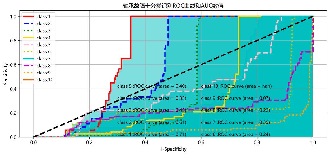
First, a crucial clarification: The AUC itself is a single number (a value between 0 and 1) that summarizes the performance of a model across all possible thresholds. It does not represent a single "best" threshold.

Instead, we use the AUC to evaluate how well our model can distinguish between classes. Then, we use other metrics (like F1-score, Youden's J statistic, or by considering business costs) to find the optimal threshold for our specific needs.

Here's a complete guide covering:

1. Understanding the ROC Curve and Thresholds
2. Finding the "Optimal" Threshold using different methods.
3. Using the Chosen Threshold to make final predictions.
4. Full Python Code Example with scikit-learn.

Understanding the ROC Curve and Thresholds

• Classifier Output: Most binary classifiers don't output a hard "0" or "1". They output a probability score (e.g., a 0.85 probability that a sample belongs to the positive class).
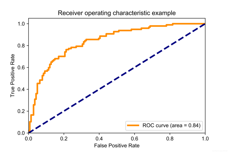
• Threshold: This probability score is then compared to a threshold. If the score is >= the threshold, the prediction is 1 (positive). Otherwise, it's 0 (negative).
• ROC Curve: This curve plots the True Positive Rate (TPR) against the False Positive Rate (FPR) for every possible threshold from 0.0 to 1.0.
  • TPR (Sensitivity/Recall): TP / (TP + FN) - What proportion of actual positives did we correctly identify?
  • FPR (1 - Specificity): FP / (FP + TN) - What proportion of actual negatives did we incorrectly identify as positive?

Each point on the ROC curve corresponds to a specific threshold. The AUC is the area under this entire curve.

Finding the "Optimal" Threshold

There's no single "best" threshold for all problems. The "best" one depends on your goal. Here are three popular methods to find a good candidate.

Method 1: Youden's J Statistic (Geometric Approach)

This is a very common and statistically sound method. It finds the threshold that maximizes the difference between the True Positive Rate and the False Positive Rate.

Youden's J = TPR - FPR

The threshold that maximizes this value is often considered a good balance between sensitivity and specificity.

Method 2: Maximizing the F1-Score

The F1-score is the harmonic mean of Precision and Recall. It's a great metric when you want a balance between the two and have imbalanced classes. We can calculate the F1-score for each threshold and pick the one with the highest value.

F1-Score = 2 (Precision Recall) / (Precision + Recall)

Method 3: Minimizing a Cost Function (Business-Driven Approach)

In a real-world scenario, the cost of a False Positive might be very different from the cost of a False Negative.

• Example (Spam Detection):
  • False Positive (FP): A legitimate email is marked as spam. This is annoying for the user.
  • False Negative (FN): A spam email lands in the inbox. This is a security risk and annoying.
  • You might decide that a FN is 10 times "costlier" than a FP.

You can define a cost function and find the threshold that minimizes it.

Cost = (Cost_FP FP) + (Cost_FN FN)

Using the Chosen Threshold

Once you've calculated your "optimal" threshold using one of the methods above, you apply it to your model's probability predictions to get the final class labels.

# model.predict_proba(X_test)[:, 1] gives you the probability of the positive class
probabilities = model.predict_proba(X_test)[:, 1]
# Your chosen optimal threshold
optimal_threshold = 0.6 
# Apply the threshold
final_predictions = (probabilities >= optimal_threshold).astype(int)

Full Python Code Example

Let's put it all together. We'll use the breast_cancer dataset from scikit-learn for a clear, runnable example.

import numpy as np
import pandas as pd
import matplotlib.pyplot as plt
from sklearn.model_selection import train_test_split
from sklearn.linear_model import LogisticRegression
from sklearn.metrics import (
    roc_curve,
    auc,
    roc_auc_score,
    f1_score,
    confusion_matrix,
    classification_report
)
# --- 1. Load Data and Train a Model ---
# Load the dataset
X, y = load_breast_cancer(return_X_y=True)
# Split data into training and testing sets
X_train, X_test, y_train, y_test = train_test_split(X, y, test_size=0.3, random_state=42, stratify=y)
# Train a Logistic Regression model
model = LogisticRegression(max_iter=10000)
model.fit(X_train, y_train)
# Get the predicted probabilities for the positive class (class 1)
y_scores = model.predict_proba(X_test)[:, 1]
# --- 2. Calculate the AUC ---
# The AUC is a single value summarizing performance across all thresholds
roc_auc = roc_auc_score(y_test, y_scores)
print(f"ROC AUC Score: {roc_auc:.4f}")
# --- 3. Find the Optimal Threshold ---
# We will explore all three methods mentioned above.
# Method 1: Youden's J Statistic
fpr, tpr, thresholds = roc_curve(y_test, y_scores)
# Calculate Youden's J statistic for each threshold
youden_j = tpr - fpr
# Find the index of the maximum J statistic
optimal_idx_youden = np.argmax(youden_j)
optimal_threshold_youden = thresholds[optimal_idx_youden]
print(f"\nOptimal Threshold (Youden's J): {optimal_threshold_youden:.4f}")
# Method 2: Maximizing the F1-Score
f1_scores = []
for threshold in thresholds:
    y_pred_temp = (y_scores >= threshold).astype(int)
    f1 = f1_score(y_test, y_pred_temp)
    f1_scores.append(f1)
# Find the index of the maximum F1 score
optimal_idx_f1 = np.argmax(f1_scores)
optimal_threshold_f1 = thresholds[optimal_idx_f1]
print(f"Optimal Threshold (Max F1-Score): {optimal_threshold_f1:.4f}")
# Method 3: Minimizing a Cost Function (Example)
# Let's assume a False Negative is 5x more costly than a False Positive
cost_fp = 1
cost_fn = 5
costs = []
for threshold in thresholds:
    y_pred_temp = (y_scores >= threshold).astype(int)
    tn, fp, fn, tp = confusion_matrix(y_test, y_pred_temp).ravel()
    total_cost = (cost_fp * fp) + (cost_fn * fn)
    costs.append(total_cost)
# Find the index of the minimum cost
optimal_idx_cost = np.argmin(costs)
optimal_threshold_cost = thresholds[optimal_idx_cost]
print(f"Optimal Threshold (Min Cost): {optimal_threshold_cost:.4f}")
# --- 4. Visualize the ROC Curve and Highlight the Optimal Threshold ---
plt.figure(figsize=(10, 8))
plt.plot(fpr, tpr, color='darkorange', lw=2, label=f'ROC curve (area = {roc_auc:.2f})')
plt.plot([0, 1], [0, 1], color='navy', lw=2, linestyle='--')
# Plot the three optimal points
plt.scatter(fpr[optimal_idx_youden], tpr[optimal_idx_youden], marker='o', color='red', label=f'Optimal (Youden) @ {optimal_threshold_youden:.2f}')
plt.scatter(fpr[optimal_idx_f1], tpr[optimal_idx_f1], marker='s', color='green', label=f'Optimal (F1) @ {optimal_threshold_f1:.2f}')
plt.scatter(fpr[optimal_idx_cost], tpr[optimal_idx_cost], marker='^', color='purple', label=f'Optimal (Cost) @ {optimal_threshold_cost:.2f}')
plt.xlim([0.0, 1.0])
plt.ylim([0.0, 1.05])
plt.xlabel('False Positive Rate')
plt.ylabel('True Positive Rate')'Receiver Operating Characteristic (ROC) Curve')
plt.legend(loc="lower right")
plt.show()
# --- 5. Use the Chosen Threshold for Final Predictions ---
# Let's use the threshold from Youden's J for our final model evaluation
final_predictions = (y_scores >= optimal_threshold_youden).astype(int)
print("\n--- Classification Report with Optimal Threshold (Youden's J) ---")
print(classification_report(y_test, final_predictions))

Summary of the Code Output